Piketty also adds colour by tying his observations to the literature written at the time (Austen, Dumas, Balzac), and how the assumptions made by the authors around how money, income and capital work are also reflected in the economic data that Piketty obtained.
Hopefully I've convinced you Piketty's programme is a worthwhile one, but that still leaves the fundamental question - is his analysis correct? That's a much harder question to answer, and to be honest I really don't feel qualified to pass judgement on the entirety of the book, other than to say it strikes me as pretty convincing from the limited amount of time I've spent on it. In an attempt to contribute in some small way to the larger conversation around Piketty's work, I thought I'd write about one specific argument that Piketty makes that I found less convincing than other parts of the book. Around 120 pages in, Piketty introduces what he calls the ‘Second Fundamental Law of Capitalism’, and this is where I started having difficulties in following his argument. The Second Fundamental Law of Capitalism The rule is defined as follows: $$ B = \frac{s} { g} $$ Where $B$ , as in Piketty’s first fundamental rule, is defined as the ratio of Capital (the total stock of public and private wealth in the economy) to Income (NNP): $$B = \frac{ \text{Capital}}{\text{Income}}$$ And where $g$ is the growth rate, and $s$ is the saving rate. Unlike the first rule which is an accounting identity, and therefore true by definition, the second rule is only true ‘in the long run’. It is an equilibrium that the market will move to over time, and the following argument is given by Piketty: “The argument is elementary. Let me illustrate it with an example. In concrete terms: if a country is saving 12 percent of its income every year, and if its initial capital stock is equal to six years of income, then the capital stock will grow at 2 percent a year, thus at exactly the same rate as national income, so that the capital/income ratio will remain stable. By contrast, if the capital stock is less than six years of income, then a savings rate of 12 percent will cause the capital stock to grow at a rate greater than 2 percent a year and therefore faster than income, so that the capital/income ratio will increase until it attains its equilibrium level. Conversely, if the capital stock is greater than six years of annual income, then a savings rate of 12 percent implies that capital is growing at less than 2 percent a year, so that the capital/income ratio cannot be maintained at that level and will therefore decrease until it reaches equilibrium.” I’ve got to admit that this was the first part in the book where I really struggled to follow Piketty’s reasoning – possibly this was obvious to other people, but it wasn’t to me! Analysis – what does he mean? Before we get any further, let’s unpick exactly what Piketty means by all the terms in his formulation of the law: Income = Net national product = Gross Net product *0.9 (where the factor of 0.9 is to account for depreciation of Capital) $g$ = growth rate, but growth of what? Here it is specifically growth in income, so while this is not exactly the same as GDP growth it’s pretty close. If we assume net exports do not change, and the depreciation factor (0.9) is fixed, then the two will be equal. $s$ = saving rate – by definition this is the ratio of additional capital divided by income. Since income here is net of depreciation, we are already subtracting capital depreciation from income and not including this in our saving rate. Let’s play around with a few values, splitting growth $g$, into per capita growth and demographic growth we get the following. Note that Total growth is simply the sum of demographic and per capita growth, and Beta is calculated from the other values using the law. 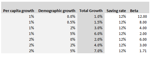
So why does Piketty introduce this law?
The argument that Piketty is intending to tease out from this equality is the following:
In fact using $g=1.5 \%$ as a long term average, we can expect Beta to crystallise around a Beta of $8$! Much higher than it has been for the past 100 years. Analysis - convergence As Piketty is quick to point out, this is a long run equilibrium towards which an economy will move. Moreover, it should be noted that the convergence of this process is incredibly slow. Here is a graph plotting the evolution of Beta, from a starting point of 5, under the assumption of $g=1.5 \%$, $s = 12 \%$: 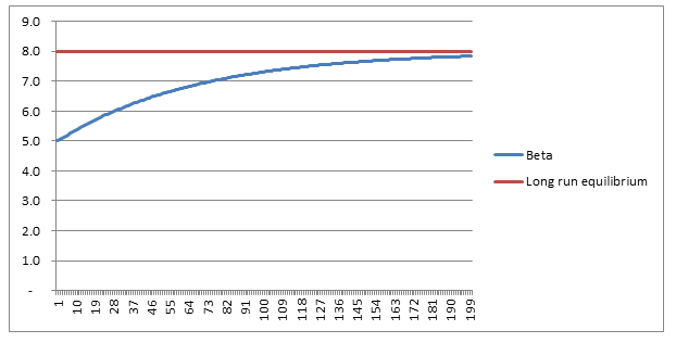
So we see that after 30 years ( i.e. approx. one generation), Beta has only increased from its starting point of $5$ to around $6$, it then takes another generation and a half to get to $7$, which is still short of its long run equilibrium of $8$.
Analysis - Is this rule true? Piketty is of course going to want to use his formula to say interesting things about the historic evolution of the Capital/Income ratio, and also use it to help predict future movements in Beta. I think this is where we start to push the boundaries of what we can easily reason, without first slowing down and methodically examining our implicit assumptions. For example – is a fixed saving rate (independent of changes in both Beta, and Growth) reasonable? Remember that the saving rate here is a saving rate on net income. So that as Beta increases, we are already having to put more money into upkeep of our current level of capital, so that a fixed net saving rate is actually consistent with an increasing gross saving rate, not a fixed gross saving rate. An increasing gross saving rate might be a reasonable assumption or it might not – this then becomes an empirical question rather than something we can reason about a priori. Another question is how the law performs for very low rates of $g$, which is in fact how Piketty is intending to use the equation. By inspection, we can see that:
As $g \rightarrow 0$, $B \rightarrow \infty $.
What is the mechanism by which this occurs in practice? It’s simply that if GDP does not grow from one year to the next, but the net saving rate is still positive, then the stock of capital will still increase, however income has not increased. This does however mean that an ever increasing share of the economy is going towards paying for capital depreciation.
Conclusion
Piketty’s law is still useful, and I do find it convincing to a first order of approximation. But I do think this section of the book could have benefited from more time spent highlighting some of the distortions potentially caused by using net income as our primary measure of income. There are multiple theoretical models used in macroeconomics, and it would have been useful for Piketty to help frame his law within the established paradigm. The Rule of 7212/1/2020 I'm always begrudgingly impressed by brokers and underwriters who can do most of their job without resorting to computers or a calculator. If you give them a gross premium for a layer, they can reel off gross and net rates on line, the implied loss cost, and give you an estimate of the price for a higher layer using an ILF in their head. When I'm working, so much actuarial modelling requires a computer (sampling from probability distributions, Monte Carlo methods, etc.) that just to give any answer at all I need to fire up Excel and make a Spreadsheet. So anytime there's a chance to do some shortcuts I'm always all for it! One mental calculation trick which is quite useful when working with compound interest is called the Rule of 72. It states that for interest rate $i$, under growth from annual compound interest, it takes approximately $\frac{72}{i} $ years for a given value to double in size. Why does it work? Here is a quick derivation showing why this works, all we need is to manipulate the exact solution with logarithms and then play around with the Taylor expansion. We are interested in the following identity, which gives the exact value of $n$ for which an investment doubles under compound interest: $$ \left( 1 + \frac{i}{100} \right)^n = 2$$ Taking logs of both sides gives the following: $$ ln \left( 1 + \frac{i}{100} \right)^n = ln(2)$$ And then bringing down the $n$: $$n* ln \left( 1 + \frac{i}{100} \right) = ln(2)$$ And finally solving for $n$: $$n = \frac {ln(2)} { ln \left( 1 + \frac{i}{100} \right) }$$ So the above gives us a formula for $n$, the number of years. We now need to come up with a simple approximation to this function, and we do so by examining the Taylor expansion denominator of the right have side: We can compute the value of $ln(2)$:
$$ln(2) \approx 69.3 \%$$
The Taylor expansion of the denominator is:
$$ln \left( 1 + \frac{i}{100} \right) = \frac{r}{100} – \frac{r^2}{20000} + … $$ In our case, it is more convenient to write this as: $$ln \left( 1 + \frac{i}{100} \right) = \frac{1}{100} \left( r – \frac{r^2}{200} + … \right) $$ For $r<10$, the second term is less than $\frac{100}{200} = 0.5$. Given the first term is of the order $10$, this means we are only throwing out an adjustment of less than $5 \%$ to our final answer. Taking just the first term of the Taylor expansion, we end up with: $$n \approx \frac{69.3 \%}{\frac{1}{100} * \frac{1}{r}}$$ And rearranging gives: $$n \approx \frac{69.3}{r}$$ So we see, we are pretty close to $ n \approx \frac{72}{r}$. Why 72? We saw above that using just the first term of the Taylor Expansion suggests we should be using the ‘rule of 69.3%' instead. Why then is this the rule of 72? There are two main reasons, the first is that for most of the interest rates we are interested in, the Rule of 72 actually gives a better approximation to the exact solution, the following table compares the exact solution, the approximation given by the ‘Rule of 69’, and the approximation given by the Rule of 72: 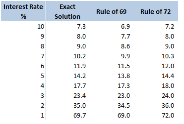
The reason for this is that for interest rates in the 4%-10% range, the second term of the Taylor expansion is not completely negligible, and act to make the denominator slightly smaller and hence the fraction slightly bigger. It turns out 72 is quite a good fudge factor to account for this.
Another reason for using 72 over other close numbers is that 72 has a lot of divisors, in particular out of all the integers within 10 of 72, 72 has the most divisors. The following table displays the divisors function d(n), for values of n between 60 and 80. 72 clearly stands out as a good candidate. 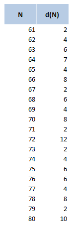
The rule of 72 in Actuarial Modelling
The main use I find for this trick is in mentally adjusting historic claims for claims inflation. I know that if I put in 6% claims inflation, my trended losses will double in size from their original level approximately every 12 years. Other uses include when analysing investment returns, thinking about the effects of monetary inflation, or it can even be useful when thinking about the effects of discounting. Can we apply the Rule of 72 anywhere else? As an aside, we should be careful when attempting to apply the rule of 72 over too long a time period. Say we are watching a movie set in 1940, can we use the Rule of 72 to estimate what values in the movie are equivalent to now? Let's set up an example and see why it doesn't really work in practice. Let's suppose an item in our movie costs 10 dollars. First we need to pick an average inflation rate for the intervening period (something in the range of 3-4% is probably reasonable). We can then reason as follows; 1940 was 80 years ago, at 4% inflation, $\frac{72}{4} = 18$, and we’ve had approx. 4 lots of 18 years in that time. Therefore the price would have doubled 4 times, or will now be a factor of 16. Suggesting that 10 dollars in 1940 is now worth around 160 dollars in today's terms. It turns out that this doesn’t really work though, let’s check it against another calculation. The average price of a new car in 1940 was around 800 dollars and the average price now is around 35k, which is a factor of 43.75, quite a bit higher than 16. The issue with using inflation figures like these over very long time periods, is for a given year the difference in the underlying goods is fairly small, therefore a simple percentage change in price is an appropriate measure. When we chain together a large number of annual changes, after a certain number of years, the underlying goods have almost completely changed from the first year to the last. For this reason, simply multiplying an inflation rate across decades completely ignores both improvements in the quality of goods over time, and changes in standards of living, so doesn't really convey the information that we are actually interested in.  Photo by David Preston What is a floating deductible? Excess of Loss contacts for Aviation books, specifically those covering airline risks (planes with more than 50 seats) often use a special type of deductible, called a floating deductible. Instead of applying a fixed amount to the loss in order to calculate recoveries, the deductible varies based on the size of the market loss and the line written by the insurer. These types of deductibles are reasonably common, I’d estimate something like 25% of airline accounts I’ve seen have had one. As an aside, these policy features are almost always referred to as deductibles, but technically are not actually deductibles from a legal perspective, they should probably be referred to as floating attachment instead. The definition of a deductible requires that it be deducted from the policy limit rather than specifying the point above which the policy limit sits. That’s a discussion for another day though! The idea is that the floating deductible should be lower for an airline on which an insurer takes a smaller line, and should be higher for an airline for which the insurer takes a bigger line. In this sense they operate somewhat like a surplus lines contract in property reinsurance. Before I get into my issues with them, let’s quickly review how they work in the first place. An example When binding an Excess of Loss contract with a floating deductible, we need to specify the following values upfront:
And we need to know the following additional information about a given loss in order to calculate recoveries from said loss:
A standard XoL recovery calculation with the fixed attachment given above, would first calculate the UNL (200m*0.75%=1.5m), and then deduct the fixed attachment from this (1.5m-1.5m=0). Meaning in this case, for this loss and this line size, nothing would be recovered from the XoL. To calculate the recovery from XoL with a floating deductible, we would once again calculate the insured’s UNL 1.5m. However we now need to calculate the applicable deductible, this will be the lesser of 1.5m (the fixed attachment), and the insurer’s effective line (defined as their UNL divided by the market loss = 1.5m/200m) multiplied by the Original Market Loss as defined in the contract. In this case, the effective line would be 0.75%, and the Original Market Loss would be 150m, hence; 0.75%*150m = 1.125m. Since this is less than the 1.5m fixed attachment, the attachment we should use is 1.125m our limit is always just 18.5m, and doesn’t change if the attachment drops down. We would therefore calculate recoveries to this contract, for this loss size and risk, as if the layer was a 18.5m xs 1.125. Meaning the ceded loss would be 0.375m, and the net position would be 1.125m. Here’s the same calculation in an easier to follow format: 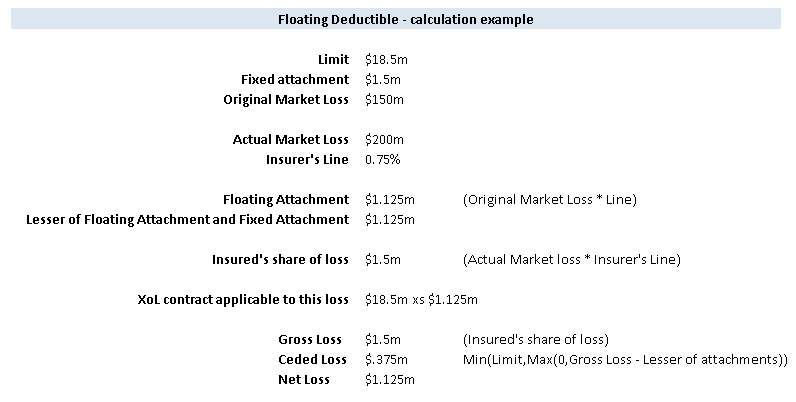 So…. what’s the issue?
This may seem quite sensible so far, however the issue is with the wording. The following is an example of a fairly standard London Market wording, taken from an anonymised slip which I came across a few years ago. Priority: USD 10,000,000 each and every loss or an amount equal to the “Reinsured’s Portion’ of the total Original Insured Loss sustained by the original insured(s) of USD 200,000,000 each and every loss, whichever the lesser. … Reinsuring Clause Reinsurers shall only be liable if and when the ultimate net loss paid by the Reinsured in respect of the interest as defined herein exceeds USD 10,000,000 each and every loss or an amount equal to the Reinsured’s Proportion of the total Original Insured Loss sustained by the original insured(s) of USD 200,000,000 or currency equivalent, each and every loss, whichever the lesser (herein referred to as the “Priority”) For the purpose herein, the Reinsured’s Proportion shall be deemed to be a percentage calculated as follows, irrespective of the attachment dates of the policies giving rise to the Reinsured’s ultimate net loss and the Original Insured Loss: Reinsured Ultimate Net Loss / Original Insured Loss … The Original Insured Loss shall be defined as the total amount incurred by the insurance industry including any proportional co-insurance and or self-insurance of the original insured(s), net of any recovery from any other source What’s going on here is that we’ve defined the effective line to be the Reinsured’s unl divided by the 100% market loss. First problem From a legal perspective, how would an insurer (or reinsurer for that matter), prove what the 100% insured market loss is? The insurer obviously knows their share of the loss, however what if this is a split placement with 70% placed in London on the same slip, 15% placed in a local market (let’s say Indonesia?), and a shortfall cover (15%) placed in Bermuda. Due to the different jurisdictions, let’s say the Bermudian cover has a number of exclusions and subjectivities, and the Indonesian cover operates under the Indonesian legal system which does not publically disclose private contract details. Even if the insurer is able to find out through a friendly broker what the other markets are paying, and therefore have a good sense of what the 100% market loss is, they may not have a legal right to this information. The airline does have a legal right to the information, however the reinsurance contract is a contract between the insured and reinsured, the airline is not a party to the reinsurance contract. The point is whether the insurer and reinsured have the legal right to the information. The above issues may sound quite theoretical, and in practice there are normally no issues with collecting on these types of contracts. But to my mind, legal language should bear up to scrutiny even when stretched – that’s precisely when you are going to rely on it. My contention is that as a general rule, it is a bad idea to rely on information in a contract which you do not have an automatic legal right to obtain. The second problem The intention with this wording, and with contracts of this form is that the effective line should basically be the same as the insured’s signed line. Assuming everything is straightforward, if the insurer takes a x% line with a limit of Y bn. If the loss is anything less than Y bn, then the insured’s effective line will simply be x%*Size of Loss / Size of loss. i.e. x%. My guess as to why it is worded this way rather than just taking the actual signed line is that we don’t want to open ourselves to a issues around what exactly we mean by ‘the signed line’ – what if the insured has exposure through two contracts both of which have different signed lines, what if there is an inuring Risk Excess which effectively nets down the gross signed line – should we then use the gross or net line? By couching the contract in terms of UNLs and Market losses we attempt to avoid these ambiguities Let me give you a scenario though where this wording does fall down: Scenario 1 – clash loss Let’s suppose there is a mid-air collision between two planes. Each results in an insured market loss of USD 1bn, then the Original Insured Loss is USD 2bn. If our insurer takes a 10% line on the first airline, but does not write the second airline, then their effective line is 10% * 1bn / 2bn = 5%... hmmm this is definitely equal to their signed line of 10%. You may think this is a pretty remote possibility, after all in the history of modern commercial aviation such an event has not occurred. What about the following scenario which does occur fairly regularly? Scenario 2 – airline/manufacturer split liability Suppose now there is a loss involving a single plane, and the size of the loss is once again USD 1bn, and that our insurer once again has a 10% line. In this case though, what if the manufacturer is found 50% responsible? Now the insurer only has a UNL of USD 500m, and yet once again, in the calculation of their floating deductible, we do the following: 10% * 500m/1bn = 5%. Hmmm, once again our effective line is below our signed line, and the floating deductible will drop down even further than intended. Suggested alternative wording My suggested wording, and I’m not a lawyer so this is categorically not legal advice, is to retain the basic definition of effective line - as UNL divided by some version of the 100% market loss - by doing so we still neatly sidestep the issues mentioned above around gross vs net lines, or exposure from multiple slips, but instead to replace the definition of Original Insured Loss with some variation of the following ‘the proportion of the Original Insured Loss, for which the insured derives a UNL through their involvement in some contract of insurance, or otherwise’. Basically the intention is to restrict the market loss, only to those contracts through which the insurer has an involvement. This deals with both issues – the insurer would not be able to net down their line further through references to insured losses which are nothing to do with them, as in the case of scenario 1 and 2 above, and secondly it restrict the information requirements to contracts which the insurer has an automatic legal right to have knowledge of since by definition they will be a party to the contract. I did run this idea past a few reinsurance brokers a couple of years ago, and they thought it made sense. The only downside from their perspective is that it makes the client's reinsurance slightly less responsive i.e. they knew about the strange quirk whereby the floating deductible dropped in the event of a manufacturer involvement, and saw it as a bonus for their client, which was often not fully priced in by the reinsurer. They therefore had little incentive to attempt to drive through such a change. The only people who would have an incentive to push through this change would be the larger reinsurers, though I suspect they will not do so until they've already been burnt and attempted to rely on the wording in a court case and, at which point they may find it does not quite operate in the way they intended. Excel Protect Sheet Encryption27/12/2019
The original idea for this post came from a slight quirk I noticed in some VBA code I was running (code pasted below) If you've ever needed to remove the protect sheet from a Spreadsheet without knowing the password, then you probably recognise it.
Sub RemovePassword()

Dim i As Integer, j As Integer, k As Integer
Dim l As Integer, m As Integer, n As Integer
Dim i1 As Integer, i2 As Integer, i3 As Integer
Dim i4 As Integer, i5 As Integer, i6 As Integer
On Error Resume Next
For i = 65 To 66: For j = 65 To 66: For k = 65 To 66
For l = 65 To 66: For m = 65 To 66: For i1 = 65 To 66
For i2 = 65 To 66: For i3 = 65 To 66: For i4 = 65 To 66
For i5 = 65 To 66: For i6 = 65 To 66: For n = 32 To 126
ActiveSheet.Unprotect Chr(i) & Chr(j) & Chr(k) & _
Chr(l) & Chr(m) & Chr(i1) & Chr(i2) & Chr(i3) & _
Chr(i4) & Chr(i5) & Chr(i6) & Chr(n)
If ActiveSheet.ProtectContents = False Then
MsgBox "Password is " & Chr(i) & Chr(j) & _
Chr(k) & Chr(l) & Chr(m) & Chr(i1) & Chr(i2) & _
Chr(i3) & Chr(i4) & Chr(i5) & Chr(i6) & Chr(n)
Exit Sub
End If
Next: Next: Next: Next: Next: Next
Next: Next: Next: Next: Next: Next
End Sub
Nothing too interesting so far, the code looks quite straight forward - we've got a big set of nested loops which appear to test all possible passwords, and will eventually brute force the password - if you've ever tried it you'll know it works pretty well. The interesting part is not so much the code itself, as the answer the code gives - the password which unlocks the sheet is normally something like ‘AAABAABA@1’. I’ve used this code quite a few times over the years, and always with similar results, the password always looks like some variation of this string. This got me thinking - surely it is unlikely that all the Spreadsheets I’ve been unlocking have had passwords of this form? So what’s going on? After a bit of research, it turns out Excel doesn’t actually store the original password, instead it stores a 4-digit hash of the password. Then to unlock the Spreadsheet, Excel hashes the password attempt and compares it to the stored hashed password. Since the size of all possible passwords is huge (full calculations below), and the size of all possible hashes is much smaller, we end up with a high probability of collisions between password attempts, meaning multiple passwords can open a given Spreadsheet. I think the main reason Microsoft uses a hash function in this way rather than just storing the unhashed password is that the hash is stored by Excel as an unencrypted string within a xml file. In fact, an .xlsx file is basically just a zip containing a number of xml files. If Excel didn't first hash the password then you could simply unzip Excel file, find the relevant xml file and read the password from any text editor. With the encryption Excel selected, the best you can do is open the xml file and read the hash of the password, which does not help with getting back to the password due to the nature of the hash function. What hash function is used? I couldn't find the name of the hash anywhere, but the following website has the fullest description I could find of the actual algorithm. As an aside, I miss the days when the internet was made up of websites like this – weird, individually curated, static HTML, obviously written by someone with deep expertise, no ads as well! Here’s the link: http://chicago.sourceforge.net/devel/docs/excel/encrypt.html And the process is as follows:
Here is the algorithm to create the hash value:
a -> 0x61 << 1 == 0x00C2 b -> 0x62 << 2 == 0x0188 c -> 0x63 << 3 == 0x0318 d -> 0x64 << 4 == 0x0640 e -> 0x65 << 5 == 0x0CA0 f -> 0x66 << 6 == 0x1980 g -> 0x67 << 7 == 0x3380 h -> 0x68 << 8 == 0x6800 i -> 0x69 << 9 == 0x5201 (unrotated: 0xD200) j -> 0x6A << 10 == 0x2803 (unrotated: 0x1A800) count: 0x000A constant: 0xCE4B result: 0xFEF1 This value occurs in the PASSWORD record.
How many trials will we need to decrypt?
Now we know how the algorithm works, can we come up with a probabilistic bound on the number of trials we would need to check in order to be almost certain to get a collision when carrying out a brute force attack (as per the VBA code above)?
This is a fairly straight forward calculation – the probability of guessing incorrectly for a random attempt is $\frac{1}{65536}$. To keep the maths simple, if we assume independence of attempts, the probability of not getting the password after $n$ attempts is simply: $$ \left( \frac{1}{65536} \right)^n$$ The following table then displays these probabilities
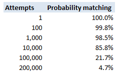
So we see that with 200,000 trials, there is a less than 5% chance of not having found a match.
We can also derive the answer directly, we are interested in the following probabilistic inequality: $$ \left( 1- \frac{1}{65536} \right)^k < 0.05$$ Taking logs of both sides gives us: $$ln \left( 1- \frac{1}{65536}\right)^k = ln( 0.05)$$ And then bringing down the k: $$k * ln \left( 1- \frac{1}{65536} \right) = ln(0.05)$$ And then solving for $k$: $$k = \frac{ ln(0.05)}{ln \left(1- \frac{1}{65536}\right)} = 196,327$$
Can I work backwards to find the password from a given hash?
As we explained above, in order to decrypt the sheet, you don’t need to find the password, you only need to find a password. Let’s suppose however, for some reason we particularly wanted to find the password which was used, is there any other method to work backwards? I can only think of two basic approaches: Option 1 – find an inversion of the hashing algorithm. Since this algorithm has been around for decades, and is designed to be difficult to reverse, and so far has not been broken, this is a bit of a non-starter. Let me know if you manage it though! Option 2 – Brute force it. This is basically your only chance, but let’s run some maths on how difficult this problem is. There are $94$ possible characters (A-Z, a-z,0-9), and in Excel 2010, the maximum password length is $255$, so in all there are, $94^{255}$ possible passwords. Unfortunately for us, that is more than the total number of atoms in the universe $(10^{78})$. If we could check $1000$ passwords per second, then it would take far longer than the current age of the universe to find the correct one. Okay, so that’s not going to work, but can we make the process more efficient? Let’s restrict ourselves to looking at passwords of a known length. Suppose we know the password is only a single character, in that case we simply need to check $94$ possible passwords, one of which should unlock the sheet, hence giving us our password. In order to extend this reasoning to passwords of arbitrary but known length, let’s think of the hashing algorithm as a function and consider its domain and range: Let’s call our hashing algorithm $F$, the set of all passwords of length $i$, $A_i$, and the set of all possible password hashes $B$. Then we have a function: $$ F: A_i -> B$$ Now if we assume the algorithm is approximately equally spread over all the possible values of $B$, then we can use the size of $B$ to calculate the size of the kernel $F^{-1}[A_i]$. The size of $B$ doesn’t change. Since we have a $4$ digit hexadecimal, it is of size $16^4$, and since we know the size of $A_i$ is $96$, we can then estimate the size of the kernel. Let’s take $i=4$, and work it through:
$A_4$ is size $96^4 = 85m$, $B = 65536$, hence $|F^{-1}[A_4]| = \frac{85m}{65536} = 124416$
Which means for every hash, there are $124,416$ possible $4$ digit passwords which can create this hash, and therefore may have been the original password. Here is a table of the values for $I = 1$ to $6$: 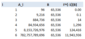
In fact we can come up with a formula for size of the kernel: $$\frac{96^i}{16^4} \sim 13.5 * 96^{i-2}$$
Which we can see quickly approaches infinity as $i$ increases. So for $i$ above $5$, the problem is basically intractable without further improvement. How would we progress if we had to? The only other idea I can come up with is to generate a huge array of all possible passwords (based on brute forcing like above and recording all matches), and then start searching within this array for keywords. We could possibly use some sort of fuzzylookup against a dictionary of keywords. If the original password did not contain any words, but was instead just a fairly random collection of characters then we really would be stumped. I imagine that this problem is basically impossible (and could probably be proved to be so using information theory and entropy) Who invented this algorithm? No idea…I thought it might be fun to do a little bit of online detective work. You see this code all over the internet, but can we find the original source? This site has quite an informative page on the algorithm: https://www.spreadsheet1.com/sheet-protection.html The author of the above page is good enough to credit his source, which is the following stack exchange page: https://superuser.com/questions/45868/recover-sheet-protection-password-in-excel Which in turns states that the code was ‘'Author unknown but submitted by brettdj of www.experts-exchange.com’ I had a quick look on Experts-exchange, but that's as far as I could get, at least we found the guy's username. Can we speed the algorithm up or improve it in any way? I think the current VBA code is basically as quick as it is going to get - the hashing algorithm should work just as fast with a short input as a 12 character input, so starting with a smaller value in the loop doesn’t really get us anything. The only real improvement I can suggest, is that if the Spreadsheet is running too slowly to be able to test a sufficient number of hashes per second, then the hashing algorithm could be implemented in python (which I started to do just out of interest, but it was a bit too fiddly to be fun). Once the algorithm is set up, the password could then be brute forced from there (in much quicker time), and one a valid password has been found, this can then be simply typed into Excel. Should I inflate my loss ratios?14/12/2019 I remember being told as a relatively new actuarial analyst that you "shouldn't inflate loss ratios" when experience rating. This must have been sitting at the back of my mind ever since, because last week, when a colleague asked me basically the same question about adjusting loss ratios for claims inflation, I remembered the conversation I'd had with my old boss and it finally clicked. Let's go back a few years - it's 2016 - Justin Bieber has a song out in which he keeps apologising, and to all of us in the UK, Donald Trump (if you've even heard of him) is still just the America's version of Alan Sugar. I was working on the pricing for a Quota Share, I can't remember the class of business, but I'd been given an aggregate loss triangle, ultimate premium estimates, and rate change information. I had carefully and meticulously projected my losses to ultimate, applied rate changes, and then set the trended and developed losses against ultimate premiums. I ended up with a table that looked something like this: (Note these numbers are completely made up but should give you a gist of what I'm talking about.) 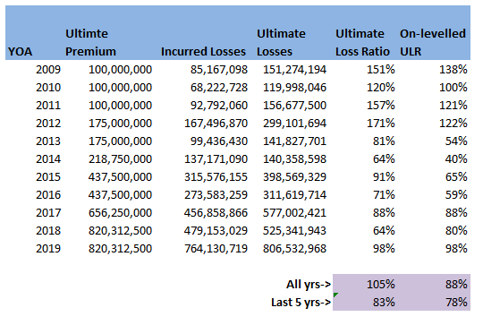
I then thought to myself ‘okay this is a property class, I should probably inflate losses by about $3\%$ pa’, the definition of a loss ratio is just losses divided by premium, therefore the correct way to adjust is to just inflate the ULR by $3\%$ pa. I did this, sent the analysis to my boss at the time to review, and was told ‘you shouldn’t inflate loss ratios for claims inflation, otherwise you'd need to inflate the premium as well’ – in my head I was like ‘hmmm, I don’t really get that...’ we’ve accounted for the change in premium by applying the rate change, claims certainly do increase each year, but I don't get how premiums also 'inflate' beyond rate movements?! but since he was the kind of actuary who is basically never wrong and we were short on time, I just took his word for it. I didn’t really think of it again, other than to remember that ‘you shouldn’t inflate loss ratios’, until last week one of my colleagues asked me if I knew what exactly this ‘Exposure trend’ adjustment in the experience rating modelling he’d been sent was. The actuaries who had prepared the work had taken the loss ratios, inflated them in line with claims inflation (what you're not supposed to do), but then applied an ‘exposure inflation’ to the premium. Ah-ha I thought to myself, this must be what my old boss meant by inflating premium. I'm not sure why it took me so long to get to the bottom of what, is when you get down to it, a fairly simple adjustment. In my defence, you really don’t see this approach in ‘London Market’ style actuarial modelling - it's not covered in the IFoA exams for example. Having investigated a little, it does seem to be an approach which is used by US actuaries more – possibly it’s in the CAS exams? When I googled the term 'Exposure Trend', not a huge amount of useful info came up – there are a few threads on Actuarial Outpost which kinda mention it, but after mulling it over for a while I think I understand what is going on. I thought I’d write up my understanding in case anyone else is curious and stumbles across this post. Proof by Example I thought it would be best to explain through an example, let’s suppose we are analysing a single risk over the course of one renewal. To keep things simple, we’ll assume it’s some form of property risk, which is covering Total Loss Only (TLO), i.e. we only pay out if the entire property is destroyed. Let’s suppose for $2018$, the TIV is $1m$ USD, we are getting a net premium rate of $1\%$ of TIV, and we think there is a $0.5\%$ chance of a total loss. For $2019$, the value of the property has increased by $5\%$, we are still getting a net rate of $1\%$, and we think the underlying probability of a total loss is the same. In this case we would say the rate change is $0\%$. That is: $$ \frac{\text{Net rate}_{19}}{\text{Net rate}_{18}} = \frac{1\%}{1\%} = 1 $$ However we would say that claim inflation is $5\%$, which is the increase in expected claims this follows from: $$ \text{Claim Inflation} = \frac{ \text{Expected Claims}_{19}}{ \text{Expected Claims}_{18}} = \frac{0.5\%*1.05m}{0.5\%*1m} = 1.05$$
From first principles, our expected gross gross ratio (GLR) for $2018$ is:
$$\frac{0.5 \% *(TIV_{18})}{1 \% *(TIV_{18})} = 50 \%$$ And for $2019$ is: $$\frac{0.5\%*(TIV_{19})}{1\%*(TIV_{19})} = 50\%$$ i.e. they are the same! The correct adjustment when on-levelling $2018$ to $2019$ should therefore result in a flat GLR – this follows as we’ve got the same GLR in each year when we calculated above from first principles. If we’d taken the $18$ GLR, applied the claims inflation $1.05$ and applied the rate change $1.0$, then we might erroneously think the Gross Loss Ratio would be $50\%*1.05 = 52.5\%$. This would be equivalent to what I did in the opening paragraph of this post, the issue being, that we haven’t accounted for trend in exposure and our rate change is a measure of the change in net rate. If we include this exposure trend as an additional explicit adjustment this gives $50\%*1.05*1/1.05 = 50\%$. Which is the correct answer, as we can see by comparing to our first principles calculation. So the fundamental problem, is that our measure of rate change is a measure in the movement of rate on TIV, whereas our claim inflation is a measure of the movement of aggregate claims. These two are misaligned, if our rate change was instead a measure in the movement of overall premium, then the two measures would be consistent and we would not need the additional adjustment. However it’s much more common in this type of situation to get given rate change as a measure of change in rate on TIV. An advantage of making an explicit adjustment for exposure trend and claims inflation is that it allows us to apply different rates – which is probably more accurate. There’s no a-priori justification as to why the two should always be the same. Claim inflation will be affected by additional factors beyond changes in the inflation of the assets being insured, this may include changes in frequency, changes in court award inflation, etc… It’s also interesting to note that the clam inflation here is of a different nature to what we would expect to see in a standard Collective Risk Model. In that case we inflate individual losses by the average change in severity i.e. ignoring any change in frequency. When adjusting the LR above, we are adjusting for both the change in frequency and severity together, i.e. in the aggregate loss. The above discussion also shows the importance of understanding exactly what someone means by ‘rate change’. It may sound obvious but there are actually a number of subtle differences in what exactly we are attempting to measure when using this concept. Is it change in premium per unit of exposure, is it change in rate per dollar of exposure, or is it even change in rate adequacy? At various points I’ve seen all of these referred to as ‘rate change’. Constructing Probability Distributions9/11/2019
There is a way of thinking about probability distributions that I’ve always found interesting, and to be honest I don’t think I’ve ever seen anyone else write about it. For each probability distribution, the CDF can be thought of as a partial infinite sum, or partial integral identity, and the probability distribution is uniquely defined by this characterisation (with a few reasonable conditions)
I think at this point most people will either have no idea what I'm talking about (probably because I've explained it badly), or they’ll think what I’ve just said is completely obvious. Let me give an example to help illustrate. Poisson Distribution as a partial infinite sum Start with the following identity:
$$ \sum_{i=0}^{\infty} \frac{ x^i}{i!} = e^{x}$$
And let's bring the exponential over to the other side. $$ \sum_{i=0}^{\infty} \frac{ x^i}{i!} e^{-x} = 1$$ Let's state a few obvious facts about this equation; firstly, this is an infinite sum (which I claimed above were related to probability distributions - so good so far). Secondly, the identity is true by the definition of $e^x$, all we need to do to prove the identity is show the convergence of the infinite sum, i.e. that $e^x$ is well defined. Finally, each individual summand is greater than or equal to 0. With that established, if we define a function: $$ F(x;k) = \sum_{i=0}^{k} \frac{ x^i}{i!} e^{-x}$$ That is, a function which specifies as its parameter the number of partial sumummads we should add together. We can see from the above identity that:
But wait, the formula for $F(x;k)$ above is actually just the formula for the CDF of a Poisson random variable! That’s interesting right? We started with an identity involving an infinite sum, we then normalised it so that the sum was equal to 1, then we defined a new function equal to the partial summation from this normalised series, and voila, we ended up with the CDF of a well-known probability distribution. Can we repeat this again? (I’ll give you a hint, we can) Exponential Distribution as a partial infinite integral Let’s examine an integral this time. We’ll use the following identity: $$\int_{0}^{ \infty} e^{- \lambda x} dx = \lambda$$ An integral is basically just a type of infinite series, so let’s apply the same process, first we normalise: $$ \frac{1}{\lambda} \int_{0}^{ \infty} e^{- \lambda x} dx = 1$$ Then define a function equal to the partial integral: $$ F(y) = \frac{1}{\lambda} \int_{0}^{ y} e^{- \lambda x} dx $$ And we've ended up with the CDF of an Exponential distribution! Euler Integral of the first kind This construction even works when we use more complicated integrals. The Euler integral of the first kind is defined as:
$$B(x,y)=\int_{0}^{1}t^{{x-1}}(1-t)^{{y-1}} dt =\frac{\Gamma (x)\Gamma (y)}{\Gamma (x+y)}$$
This allows us to normalise:
$$\frac{\int_{0}^{1}t^{{x-1}}(1-t)^{{y-1}}dt}{B(x,y)} = 1$$ And once again, we can construct a probability distribution: $$B(x;a,b) = \frac{\int_{0}^{x}t^{{a-1}}(1-t)^{{b-1}}dt}{B(a,b)}$$ Which is of course the definition of a Beta Distribution, this definition bears some similarity to the definition of an exponential distribution in that our normalisation constant is actually defined by the very integral which we are applying it to. Conclusion So can we do anything useful with this information? Well not particularly. but I found it quite insightful in terms of how these crazy formulas were discovered in the first place, and we could potentially use the above process to derive our own distributions – all we need is an interesting integral or infinite sum and by normalising and taking a partial sum/integral we've defined a new way of partitioning the unit interval. Hopefully you found that interesting, let me know if you have any thoughts by leaving a comment in the comment box below! Beta Distribution in Actuarial Modelling3/11/2019
I saw a useful way of parameterising the Beta Distribution a few weeks ago that I thought I'd write about.
The standard way to define the Beta is using the following pdf:
$$f(x) = \frac{x^{\alpha -1} {(1-x)}^{\beta -1}}{B ( \alpha, \beta )}$$
Where $ x \in [0,1]$ and $B( \alpha, \beta ) $ is the Beta Function:
$$ B( \alpha, \beta) = \frac{ \Gamma (\alpha ) \Gamma (\beta)}{\Gamma(\alpha + \beta)}$$
When we use this parameterisation, the first two moments are:
$$E [X] = \frac{ \alpha}{\alpha + \beta}$$
$$Var (X) = \frac{ \alpha \beta}{(\alpha + \beta)^2(\alpha + \beta + 1)}$$
We see that the mean and the variance of the Beta Distribution depend on both parameters - $\alpha$ and $\beta$. If we want to fit these parameters to a data set using a method of moments then we need to use the following formulas, which are quite complicated:
$$\hat{\alpha} = m \Bigg( \frac{m (1-m) }{v} - 1 \Bigg) $$
$$\hat{\beta} = (1- m) \Bigg( \frac{m (1-m) }{v} - 1 \Bigg) $$ This is not the only possible parameterisation of the Beta Distribution however. We can use an alternative definition where we define:
$$\gamma = \frac{ \alpha}{\alpha + \beta} $$, and $$\delta = \alpha + \beta$$
And then by construction, $E[X] = \gamma$, and we can calculate the new variance:
$$V = \frac{ \alpha \beta}{(\alpha + \beta)^2(\alpha + \beta + 1)} = \frac{\gamma ( 1 - \gamma)}{(1-\delta)}$$.
Placing these new variables back in our pdf gives the following equation:
$$f(x) = \frac{x^{\gamma \delta -1} {(1-x)}^{\delta (1-\gamma) -1}}{B ( \gamma \delta, \delta (1-\gamma) -1 )}$$
So why would we bother to do this? Our new formula now looks more complicated to work with than the one we started with. There are however two main advantages to this new version, firstly the method of moments is much simpler to set up, our first parameter is simply the mean, and the formula for variance is easier to calculate than before. This makes using the Beta distribution much easier in a Spreadsheet. The second advantage, and in my mind the more important point, is that since we now have a strong link between the central moments and the two parameters that define the distribution we now have an easy and intuitive understand of what our parameters actually represent. As I’ve written about before, rather than just sticking with the standard statistics textbook version, I’m a big fan of pushing parameterisations that are both useful and easily interpretable, The version of the Beta Distribution presented above achieves this. Furthermore it also fits nicely with the schema I've written about before (most recently in the in the post below on negative binomial distribution), in which no matter which distribution we are talking about, the first parameter of a distribution gives you information about it's mean, the second parameter gives information about its volatility, etc. By doing this you give yourself the ability to compare distributions and sense check parameterisations at a glance. Pensions and Tax12/10/2019 Pensions and tax you think to yourself - he’s managed to find the two most boring subjects possible and now he appears to be planning to write about a combination of them! Is this some sort of attempt to win an award for the most boring and tedious blog post every? Well what if I told you this blog post, whilst being about pension and tax was also about a burning social justice, about high finance, and about death? Would you find that interesting? Okay, so I may got slightly carried away in that last paragraph and over sold slightly. This is less of a 'burning social injustice', and more an 'unfair outcome' which happens to only affect people who are already well off - but someone has to write about this stuff right? And the current status quo is genuinely unfair I promise. Lifetime Allowance Before diving into the unfairness I mentioned earlier, we need to briefly set the scene. Let’s think about all the types of tax that the government levies on us; we get taxed on our income (income tax), we get taxed on our property wealth (council tax), we get taxed on our wealth when we die (inheritance tax), and we get taxed when we buy things (VAT and other sales taxes). Since the government taxes just about every financial transaction we make, they can tweak all these different types of tax to incentivise and disincentivizes certain behaviours. One thing governments have traditionally been very keen on incentivising is getting its citizens saving enough for retirement. The way this has historically been done is to allow income tax relief on the proportion of an employee’s gross salary which is put into a pension. i.e. If you earn £30,000 and put £5,000 of that into a pension, then you pay no tax on the £5,000 and are then taxed as if you only earn £25,000. You might think to yourself great, so now people are saving more for their retirement and everyone lives happily ever after, the end. Well not quite. The problem with this arrangement is certain unscrupulous individuals started to use this mechanism to avoid paying tax. Let’s say you’re 64, quite well off, and hoping to retire next year, why not chuck most of your money into your pension? You can live off your savings for a year and then all that money you would have taken as income and therefore been taxed on can instead be deferred for a year, taken as pension when you retire, and you would pay no income tax on that year's salary. Or let’s suppose an individual come from a very wealthy family, and doesn't really need to get paid a salary to live on, then they could just put their entire salary into a pension, not take anything until they retire (at 55), and then not pay any tax at all on their earnings from their job across their entire career. Okay, fine, it sounds like we’re going to need some caps on the maximum pension tax relief to stop people doing this. Let’s say – £225k per annum is the maximum that can be put into a pension pot per year, and £1.5m is the total size of a pension pot you can build up before we start making people pay tax. That’s a large amount of money, who’s going to complain about that? These were the levels set by Tony Blair’s government between 2004 and 2006. These caps were then slowly increased over time, reaching a height of around £250k pa, and £1.8m as a lifetime allowance in 2011. These are very big figures, and it’s hard to imagine anyone objecting to a tax on an annual pension contribution above £250k. In 2011, with a rapidly expanding budget deficit to deal with and a promise to balance the books, the Conservative government instigated their infamous austerity programme. The tories had pledged to ring-fence certain areas of government spending (the NHS, and Education for example), they therefore started to look around for other areas to raise additional income which had not traditionally been taped. Tax relief for high earners seemed like an obvious target, and who can really say that the rich should not have to pay additional tax given the situation to help try to protect spending on areas such as policing or social care. By 2014 the annual allowance (the amount that can be saved per annum) had been reduced to £40k per annum, and the lifetime allowance was down to £1m. These values still seem high, however with the economy in the state it was, they are perhaps not as high as they first appear. This reduction came during a period of all-time low interest rates, I'm going to demonstrate which this caused issued by examining a series of graphs. The following graph displays the Bank of England base rate for the last twenty years, notice the significant reduction in 2007 following the global financial crisis. Note we have been at this very low level ever since. 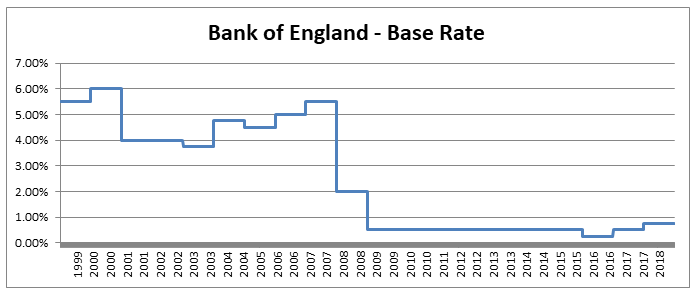 As a proxy for the investment return a pension or life insurance company could receive on a long term almost risk-free investment I’m going to use Base rate + 2%, I've plotted this as well on the graph below: 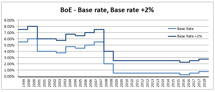 Okay, so why is this important? The interesting idea is that the ‘price’ of an annuity can be approximated using quite a simple formula. It is (very) roughly equal to: $ A = \frac{1}{i} $ Where i is our investment return. What does this mean in real numbers? If I want to retire and get a pension of £10,000 per annum, Then the price of that is going to be 10,000 * A = 10,000 / i. If i=10%, then I will need to have a pot of £100,000. If i = 1%, then I will need a pot of £1m. Let’s plot the implied annuity price on the same chart as a secondary axis: 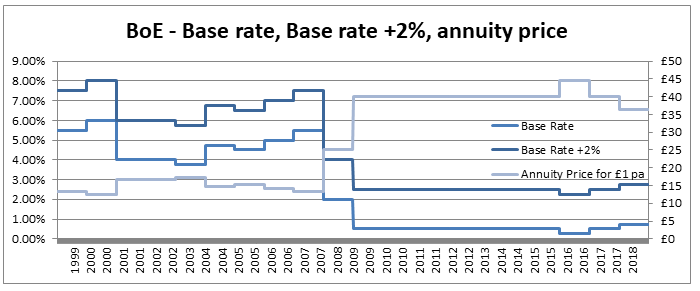 So we see we have this reciprocal relationship, as interest rates go down, the cost of an annuity goes up. At the moment, due to the very low interest rates, it costs something like £37 to purchase an annuity of £1 per annum for life. Interesting you might (or might not) think. But this annuity price becomes useful if we combine it with the lifetime tax-free allowance. If we assume a potential retiree is going to use their pension pot to purchase an annuity, then to calculate the level of pension they will be able to get, we need to take their pension pot and divide by the cost of the annuity. The graph below shows the approximate tax-free pension one could expect if retiring with a pension pot equal to the full Lifetime allowance, using the prevailing annuity rates which are in turn based on the prevailing interest rates. 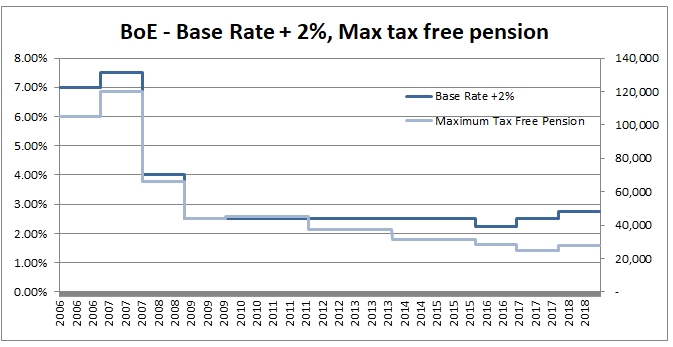 So we see that through a combination of the LTA being reduced significantly and interest rates bottoming out, we are now in the position where the maximum tax-free pension (based on approximate annuity rates) is as little as £25k. A far cry from the approximately £100k when the rule was first implemented. What about that burning social injustice you mentioned? But at least we are all treated the same right? Well not exactly… all of the above glossed over one quite important point, it assumes that the individual in question has a defined contribution pension. For individuals with a final salary pension (which includes MPs, Judges, a majority of CEOs and senior public sector employees), the LTA is calculated with reference to a fixed annuity factor of 20. Given the actual average annuity price is more like 40, this has a massive impact. Let’s plot this on a graph as well. 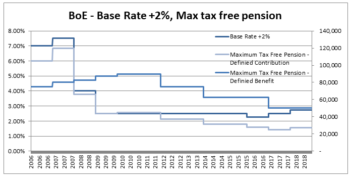 Hmmm, so we see that in 2006 when the LTA was first set up, this factor of 20 was quite generous to Defined Contribution pension holders, they could often retire with a pension of around £120k without paying any tax, whereas a defined benefit pension holder could only retire with a maximum of approx. £80k. This has now flipped, due to changes in annuity rates, and the fact that this factor has not been adjusted for so long. Under current conditions, the maximum pension that can be taken tax free is around £25k pa for a definied contribution pension, but around £50k pa for a definied benefit pension.
So what is the point of all this? What am I advocating? To me it seems clear that we need (approximate) equality of outcome in terms of taxation for defined contribution pensions compared to defined benefit schemes. This could be achieved in one of two ways, either we apply some sort of floor to how low the tax free pension can reduced to for defined contribution pensions, or we adjust the defined benefit annuity factor periodically to keep it roughly in line with market conditions and therefore apply a lower maximum tax free rate to defined benefit pensioners. This would correct the current system by which judges and MPs (and other people with DB pensions) get significant tax breaks at retirement compared to individuals with DC pensions. Negative Binomial in VBA21/9/2019
Have you ever tried to simulate a negative binomial random variable in a Spreadsheet?
If the answer to that is ‘nope – I’d just use Igloo/Metarisk/Remetrica’ then consider yourself lucky! Unfortunately not every actuary has access to a decent software package, and for those muddling through in Excel, this is not a particularly easy task. If on the other hand your answer is ‘nope – I’d use Python/R, welcome to the 21st century’. I’d say great, I like using those programs as well, but sometimes for reasons out of your control, things just have to be done in Excel. This is the situation I found myself in recently, and here is my attempt to solve it: Attempt 0 The first step I took in attempting to solve the problem was of course to Google it, then cross my fingers and hope that someone else has already solved it and this is just going to be a simple copy and paste. Unfortunately when I did search for VBA code to generate a negative binomial random variable, nothing comes up. In fact, nothing comes up when searching for code to simulate a Poisson random variable in VBA. Hopefully if you've found your way here, looking for this exact thing, then you're in luck, just scroll to the bottom and copy and paste my code. When I Googled it, there were a few solutions that almost solved the problem; there is a really useful Excel add-in called ‘Real statistics’ which I’ve used a few times: http://www.real-statistics.com/ It's a free excel add-in, and it does have functionality to simulate negative bimonials. If however you need someone to be able to re-run the Spreadsheet, they also will need to have it installed. In that case, you might as well use Python, and then hard code the frequency numbers. Also, I have had issues with it slowing Excel down considerably, so I decided not to use this in this case. I realised I’d have to come up with something myself, which ideally would meet the following criteria
How hard can that be? Attempt 1 I’d seen a trick before (from Pietro Parodi’s excellent book ‘Pricing in General Insurance’) that a negative binomial can be thought of as a Poisson distribution with a Gamma distribution as the conjugate prior. See the link below for more details: https://en.wikipedia.org/wiki/Conjugate_prior#Table_of_conjugate_distributions Since Excel has a built in Gamma inverse, we have simplified the problem to needing to write our own Poisson inverse. We can then easily generate negative binomials using a two step process:
Great, so we’ve reduced our problem to just being able to simulate a Poisson in VBA. Unfortunately there’s still no built in Poisson inverse in Excel (or at least the version I have), so we now need a VBA based method to generate this. There is another trick we can use for this - which is also taken from Pietro Parodi - the waiting time for a Poisson dist is an Exponential Dist. And the CDF of an Exponential dist is simple enough that we can just invert it and come up with a formula for generating an Exponential sample. We then set up a loop and add together exponential values, to arrive at Poisson sample. The code for this is give below:
Function Poisson_Inv(Lambda As Double)

    s = 0
    N = 0
    Do While s < 1
        u = Rnd()
        s = s - (Application.WorksheetFunction.Ln(u) / Lambda)
        k = k + 1
    Loop
    Poisson_Inv = (k - 1)

End Function
The VBA code for our negative binomial is therefore:
Function NegBinOld2(b, r)

    Dim Lambda As Double
    Dim N As Long

    u = Rnd()

    Lambda = Application.WorksheetFunction.Gamma_Inv(u, r, b)

    N = Poisson_Inv(Lambda)

    NegBinOld2 = N

End Function
Does this do everything we want?
There are a couple of downside of though:
This leads us on to Attempt 2 Attempt 2 If we pass the VBA a random uniform sample, then whenever we hit refresh in the Spreadsheet the random sample will refresh, which will force the Negative Binomial to resample. Without this, sometimes the VBA will function will not reload. i.e. we can use the sample to force a refresh whenever we like. Adapting the code gives the following:
Function NegBinOld(b, r, Rnd1 As Double)

    Dim Lambda As Double
    Dim N As Long

    u = Rnd1

    Lambda = Application.WorksheetFunction.Gamma_Inv(u, r, b)

    N = Poisson_Inv(Lambda)

    NegBinOld = N

End Function
So this solves the refresh problem. What about the random seed problem? Even though we now always get the same lambda for a given rand – and personally I quite like to hardcode these in the Spreadsheet once I’m happy with the model, just to speed things up. We still use the VBA rand function to generate the Poisson, this means everytime we refresh, even when passing it the same rand, we will get a different answer and this answer will be non-replicable. This suggests we should somehow use the first random uniform sample to generate all the others in a deterministic (but still pseudo-random) way. Attempt 3 The way I implemented this was to the set the seed in VBA to be equal to the uniform random we are passing the function, and then using the VBA random number generator (which works deterministically for a given seed) after that. This gives the following code:
Function NegBin(b, r, Rnd1 As Double)

    Rnd (-1)
    Randomize (Rnd1)

    Dim Lambda As Double
    Dim N As Long

    u = Rnd()

    Lambda = Application.WorksheetFunction.Gamma_Inv(u, r, b)

    N = Poisson_Inv(Lambda)

    NegBin = N

End Function
So we seem to have everything we want – a free, quick, solution that can be bundled in a Spreadsheet, which allows other people to rerun without installing any software, and we’ve also eliminated the forced refresh issue. What more could we want? The only slight issue with the last version of the negative binomial is that our parameters are still specified in terms of ‘b’ and ‘r’. Now what exactly are ‘b’ and ‘r’ and how do we relate them to our sample data? I’m not quite sure.... The next trick is shamelessly taken from a conversation I had with Guy Carp’s chief Actuary about their implementation of severity distributions in MetaRisk. Attempt 4 Why can't we reparameterise the distribution using parameters that we find useful, instead of feeling bound by using the standard statistics textbook definition (or even more specifically the list given in the appendix to ‘Loss Models – from data to decisions’, which seems to be somewhat of an industry standard), why can't we redefine all the parameters from all common actuarial distributions using a systematic approach for parameters? Let's imagine a framework where no matter which specific severity distribution you are looking at, the first parameter contains information about the mean (even better if it is literally scaled to the mean in some way), the second contains information about the shape or volatility, the third contains information about the tail weight, and so on. This makes fitting distributions easier, it makes comparing the goodness of fit of different distributions easier, and it make sense checking our fit much easier. I took this idea, and tied this in neatly to a method of moments parameterisation, whereby the first value is simply the mean of the distribution, and the second is the variance over the mean. This gives us our final version:
Function NegBin(Mean, VarOMean, Rnd1 As Double)

    Rnd (-1)
    Randomize (Rnd1)

    Dim Lambda As Double
    Dim N As Long

    b = VarOMean - 1
    r = Mean / b

    u = Rnd()

    Lambda = Application.WorksheetFunction.Gamma_Inv(u, r, b)

    N = Poisson_Inv(Lambda)

    NegBin = N

End Function

Function Poisson_Inv(Lambda As Double)

    s = 0
    N = 0
    Do While s < 1
        u = Rnd()
        s = s - (Application.WorksheetFunction.Ln(u) / Lambda)
        k = k + 1
    Loop
    Poisson_Inv = (k - 1)

End Function
Poisson Distribution for small Lambda23/4/2019
I was asked an interesting question a couple of weeks ago when talking through some modelling with a client.
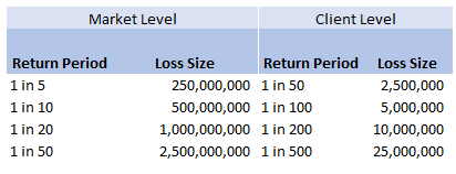
We were modelling an airline account, and for various reasons we had decided to base our large loss modelling on a very basic top-down allocation method. We would take a view of the market losses at a few different return periods, and then using a scenario approach, would allocate losses to our client proportionately. Using this method, the frequency of losses is then scaled down by the % of major policies written, and the severity of losses is scaled down by the average line size. To give some concrete numbers (which I’ve made up as I probably shouldn’t go into exactly what the client’s numbers were), let's say the company was planning on taking a line on around 10% of the Major Airline Risks, and their average line was around 1%. We came up with a table of return periods for market level losses. The table looked something like following (the actual one was also different to the table below, but not miles off): 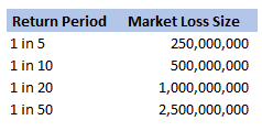
Then applying the 10% hit factor if there is a loss, and the 1% line written, we get the following table of return periods for our client:
Hopefully all quite straightforward so far. As an aside, it is quite interesting to sometimes pare back all the assumptions to come up with something transparent and simple like the above. For airline risks, the largest single policy limit is around USD 2.5bn, so we are saying our worst case scenario is a single full limit loss, and that each year this has around a 1 in 50 chance of occurring. We can then directly translate that into an expected loss, in this case it equates to 50m (i.e. 2.5bn *0.02) of pure loss cost. If we don't think the market is paying this level of premium for this type of risk, then we better have a good reason for why we are writing the policy!
So all of this is interesting (I hope), but what was the original question the client asked me? We can see from the chart that for the market level the highest return period we have listed is 1 in 50. Clearly this does translate to a much longer return period at the client level, but in the meeting where I was asked the original question, we were just talking about the market level. The client was interested in what the 1 in 200 at the market level was and what was driving this in the modelling. The way I had structured the model was to use four separate risk sources, each with a Poisson frequency (lambda set to be equal to the relevant return period), and a fixed severity. So what this question translates to is, for small Lambdas $(<<1)$, what is the probability that $n=2$, $n=3$, etc.? And at what return period is the $n=2$ driving the $1$ in $200$? Let’s start with the definition of the Poisson distribution: Let $N \sim Poi(\lambda)$, then: $$P(N=n) = e^{-\lambda} \frac{ \lambda ^ n}{ n !} $$ We are interested in small $\lambda$ – note that for large $\lambda$ we can use a different approach and apply sterling’s approximation instead. Which if you are interested, I’ve written about here: www.lewiswalsh.net/blog/poisson-distribution-what-is-the-probability-the-distribution-is-equal-to-the-mean
For small lambda, the insight is to use a Taylor expansion of the $e^{-\lambda}$ term. The Taylor expansion of $e^{-\lambda}$ is:
$$ e^{-\lambda} = \sum_{i=0}^{\infty} \frac{\lambda^i}{ i!} = 1 - \lambda + \frac{\lambda^2}{2} + o(\lambda^2) $$
We can then examine the pdf of the Poisson distribution using this approximation: $$P(N=1) =\lambda e^{-\lambda} = \lambda ( 1 – \lambda + \frac{\lambda^2}{2} + o(\lambda^2) ) = \lambda - \lambda^2 +o(\lambda^2)$$
as in our example above, we have:
$$ P(N=1) ≈ \frac{1}{50} – {\frac{1}{50}}^2$$
This means that, for small lambda, the probability that $N$ is equal to $1$ is always slightly less than lambda. Now taking the case $N=2$: $$P(N=2) = \frac{\lambda^2}{2} e^{-\lambda} = \frac{\lambda^2}{2} (1 – \lambda +\frac{\lambda^2}{2} + o(\lambda^2)) = \frac{\lambda^2}{2} -\frac{\lambda^3}{2} +\frac{\lambda^4}{2} + o(\lambda^2) = \frac{\lambda^2}{2} + o(\lambda^2)$$
So once again, for $\lambda =\frac{ 1}{50}$ we have:
$$P(N=2) ≈ 1/50 ^ 2 /2 = P(N=1) * \lambda / 2$$
In this case, for our ‘1 in 50’ sized loss, we would expect to have two such losses in a year once every 5000 years! So this is definitely not driving our 1 in 200 result.
We can add some extra columns to our market level return periods as follows: 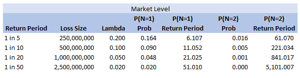
So we see for the assumptions we made, around the 1 in 200 level our losses are still primarily being driven by the P(N=1) of the 2.5bn loss, but then in addition we will have some losses coming through corresponding to P(N=2) and P(N=3) of the 250m and 500m level, and also combinations of the other return periods.
So is this the answer I gave to the client in the meeting? …. Kinda, I waffled on a bit about this kind of thing, but then it was only after getting back to the office that I thought about trying to breakdown analytically which loss levels we can expect to kick in at various return periods. Of course all of the above is nice but there is an easier way to see the answer, since we’d already stochastically generated a YLT based on these assumptions, we could have just looked at our YLT, sorted by loss size and then gone to the 99.5 percentile and see what sort of losses make up that level. The above analysis would have been more complicated if we have also varied the loss size stochastically. You would normally do this for all but the most basic analysis. The reason we didn’t in this case was so as to keep the model as simple and transparent as possible. If we had varied the loss size stochastically then the 1 in 200 would have been made up of frequency picks of various return periods, combined with severity picks of various return periods. We would have had to arbitrarily fix one in order to say anything interesting about the other one, which would not have been as interesting. Gaming my office's Cheltenham Sweepstake31/3/2019 Every year we have an office sweepstake for the Cheltenham horse racing festival. Like most sweepstakes, this one attempts to remove the skill, allowing everyone to take part without necessarily needing to know much about horse racing. In case you’re not familiar with a Sweepstake, here’s a simple example of how one based on the World Cup might work:
Note that in order for this to work properly, you need to ensure that the team draw is not carried out until everyone who wants to play has put their money in – otherwise you introduce some optionality and people can then decide whether to enter based on the teams that are still left. i.e. if you know that Germany and Spain have already been picked then there is less value in entering the competition. The rules for our Cheltenham sweepstake were as follows: The Rules The festival comprises 7 races a day for 4 days, for a total of 28 races. The sweepstake costs £20 to enter, and the winnings are calculated as follows: 3rd place in competition = 10% of pot 2nd place in competition = 20% of pot 1st place in competition = 70% of pot Each participant picks one horse per race each morning. Points are then calculated using the following scoring system:
A running total is kept throughout the competition, and the winner is determined after the final race. The odds the scoring are based on are set using the odds printed in the Metro Newspaper on the morning of the races. (as an example, for a horse which has odds of 11/2 in the Metro - if the horse then places 1st, if we selected this horse, we would win (1+11/2)*5 = 32.5 points) Initial thoughts Any set of betting odds can be converted to an implied probability of winning, these would be the odds which over the long run would cause you to breakeven if the race were repeated multiple times with each horse winning a proportion equal to its probability of winning. Because the scoring in our sweepstake is based on the betting odds, using implied probabilities derived from the odds to help select our horses ends up cancelling itself out (which was the intention when designing the rules). The implied probability can be calculated as one over the odds As an aside, the bookie is indifferent to whether this is the correct probability of winning, they structures the odds purely on the ratio of how their customers are betting. They then structure the odds so that they make money on each race, regardless of which horse wins, for an explanation of this, see my post on creating a Dutchbook: www.lewiswalsh.net/blog/archives/12-2017 Here is an example showing how we would calculate the implied probabilities using some made up odds: 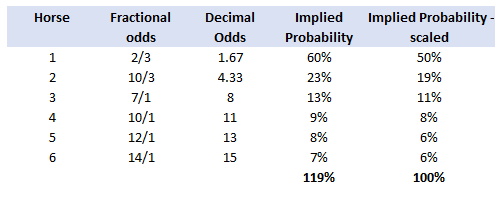 We can then use the implied probabilities we just calculated to see what would happen if each horse finished in the first three positions. Once we have done this, we can then calculate the Expected Value of betting on each horse: 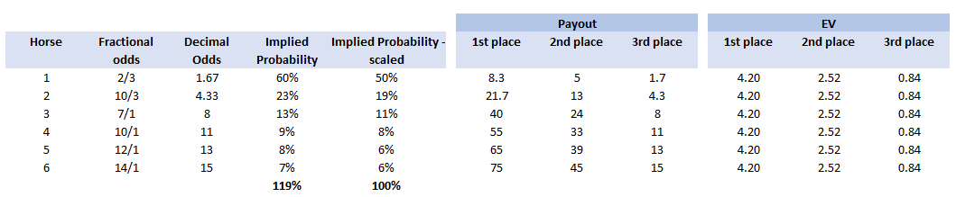 We see that the payout varies for each horse, but the EV is the same. This is by design, the intention is that it should not matter which horse you bet on, the sweepstake rules equalise everyone. So what can we - an actuary who knows nothing much about horse racing - do? I don’t have any special knowledge that would allow me to select a horse which would beat the odds listed in the Metro, we appear to be at an impasse. I could attempt to build a model of which horse will win, and then select my horse based on that, but unless it proves to be more accurate than the Metro odds, I might as well just pick at random. Furthermore, if I could build such a model, then I could just start betting actual money. This probably shows you what a difficult problem this is! There's no such thing as free money. It would be a cool project to try, and it’s something I’ve been meaning to attempt for a while, but that’s best saved for another day. Attempt 1 - Metro vs pre-race odds My first thought was that we can exploit the difference in odds between those published in the Metro in the morning, and the latest odds published closer to the start of the race. It seems reasonable to assume that the odds just before the race should be more accurate than the metro odds. There will have been time for additional information to be included in the more up to date odds, e.g. the weather is worse than expected therefore horse x is expected to be slower than usual. Since the payout will be based on the Metro, we will then be able to maximise our EV by exploiting this differential. Our table will end up looking something like this: 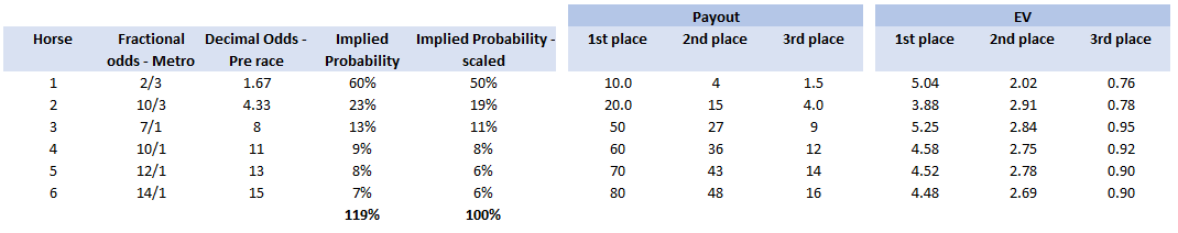 We see that we have very small variations in the EVs for some of the horses. It looks like according to this analysis Horse 3 would be the best selection as it has the highest EVs for 1st, 2nd, and 3rd. Based on this strategy, we would then go through each race and select the horse with the highest EV. Is this what I did? No, for a couple of reasons. The biggest issue was that the Metro did not publish odds in the morning for all races, meaning we couldn’t use the Metro, and therefore the rules of the sweepstake were amended to use the official pre-race odds to calculate the payout instead. This meant there was only one set of odds used, and our edge disappeared! Even if we had used this method, there was a more fundamental issue - the margins we ended up with were tiny anyway. The Metro vs pre-race odds did not swing wildly, meaning that even selecting the horse with the highest EV were only marginally better than picking at random. So, was there an alternative? Attempt 2 - 2nd and 3rd place odds My next attempt at an exploitative strategy was based on the insight that the payout multiplier for 2nd and 3rd place was based on the odds of the horse coming 1st, rather than the odds of the horse coming 2nd or 3rd. The expected value of a horse was not quite as I calculated above, it was actually: $$EV = P(1)*p_1 + P(2)*p_2 + P(3)*p_3$$ Above, we were using the implied probability of the horse coming first as a proxy for the probability it would come second and third. This is not the same, and some betting websites do allow you to bet on whether a horse will come 2nd or 3rd. For websites that do not allow you to bet directly on this, then we may still be able to calculate it from the odds for whether a horse finishes in the top 2 or 3 places. We just need to subtract out the implied probability of coming 1st from the probability of coming in the top 2, and then subtracting this out from coming top 3 etc. I therefore added some more columns to my table above, corresponding to the probability of the horses coming 2nd and 3rd, and then used this to calculate the EV instead. 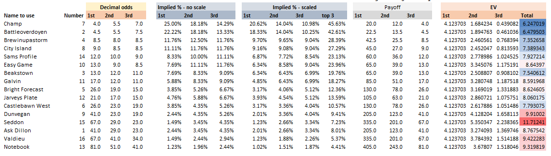 We see that the final column, Total EV, now has quite different values for each horse. In this case Horse 15, Seddon has an EV of 11.72. The favourite horse on the other hand - number 7 - only has an EV of 6.2. The intuitive explanation of this is that the probability of Seddon coming first is very low – this is the reflected in the long odds of 67, this then gives us a large multiplier, but the odds of the horse coming second or third are actually relatively less far out – the fact that it is not the favourite actually increases the odds of it coming in a position which is not 1st. But then if does come in 2nd or 3rd, we would still apply the same large multiplier for the odds of it coming 1st. This then gives us our 2nd edge – we can gain a positive EV by focusing. As a thought experiment, imagine we have a race with three horses – horse A is a clear favourite, horse B is an average horse, and horse C is clearly the weakest. By betting on horse C – the odds of it winning should be very low, so the multiple should be very high, but then this multiple will be applied even if it comes 2nd or 3rd, which is exactly where it is expected to finish. This therefore suggests our next potential strategy – select horses which maximise our EV using the implied probabilities of the horses coming 2nd, 3rd etc. So is this what I did? Well kind of.... The issue with this approach is that typically the horses that provide the best EV also have very long odds. In the race analysed above, our horse has an EV of 11.7, but it only has a 7% chance overall of coming in the top 3. In race two for example, the horse with the best EV actually only had a 2.7% chance of coming in the top 3. Since there are only 28 races in total, if each horse we selected only had a 2.7% chance of coming in, then the probability of us getting 0 points overall in the entire competition would then be: $(1-2.7 \%)^{28} = 48 \%$ So there is roughly a 50% chance we will get 0 points! Alternatively, if we selected the favourite every time, we could expect it to come top 3 almost every time, and thereby guarantee ourselves points most races, but it also has the lowest EV. So we have what appears to be a risk vs reward trade off. Pick outsiders and give ourselves the highest EV overall, or pick the favourites thereby reducing our overall EV but also reducing our volatility. This leads us neatly to attempt 3 - trying to think about how to maximise our probability of winning the competition rather than simply maximising EV for each race. Attempt 3 - EP curves From the work above, we now have our model of the position each horse will finish in each race – using the 1st, 2nd, and 3rd implied probabilities - and we have the payout for each horse – using the odds of the horse coming 1st. We can then bring our selection of horse and these probabilities together in a summary tab and simulate our daily score stochastically using a Monte Carlo method. To do this we just need to turn the implied probabilities into a CDF, and lookup the value of each position and repeat 10,000 times. The output for this then ends up looking like the following, where the value is the number of points we will for a given race. 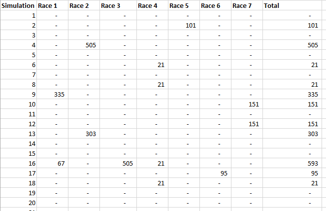 So we see that across this sample of 20 simulations, most days we to end up with 0 points overall, but a few days have very high scores. So far so good! The next step is to set up an EP table of the following, which looks like the following: 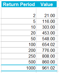 The EP table gives us the probability of exceeding various scores in the competition based on our horse selections. In this case, we see that there is a 1 in 20 chance of getting 453 points or greater in the day. This is useful even on its own – when I was deciding which horses to bet on, I simply played around with the selections until I got an EP table I was comfortable with. My reasoning was quite basic – I decided I wanted to maximise the 1 in 20 value. I wanted to give myself something like a 1/4 chance of winning the whole competition and a 3/4 chance of getting very few points. Since there were four days of races, dividing the 1/4 by another 4 suggests we should be looking at maximising the 1 in 20 level (I admit this reasoning was a bit rough, but it seemed to serve its purpose) The insight here is that the payout structure of the sweepstake is such that coming in the top 3 is all that matters, and in particular coming 1st is disproportionately rewarded. To see this, we can think of the daily selection of horses as attempting to maximise the EV of the overall prize rather than the EV of our overall score - maximising the EV of each race is only a means to this end. So we are actually interested in maximising the following: $0.7 * P(1st) + 0.2 + P(2nd) + 0.1 * P(3rd)$ Which will largely be dominated by P(1st), given the $0.7$ factor. This is largely the strategy I went for in the end. Attempt 4 - Game theory? I’ve brushed over one difficulty above; in order to maximise our prize EV we need to consider not just which strategy we should take, but how this strategy will fare against the strategies that other people will take. If everyone is maximising their 1 in 20 return period then there’s little point us doing exactly the same. Luckily for me, most people were doing little more than picking horses randomly. We could then formalise this assumption, and come up with a numerical solution to the problem above. To do this, we would simulate our returns for each day across 10,000 simulations as above, but this time we would compare ourselves against a ‘base strategy’ of random selection of horses and we would simulate this base strategy for the approximately 40 people who entered. Each simulation would then give us a ranking we would finish in the competition, Here is an example of what that would look like: 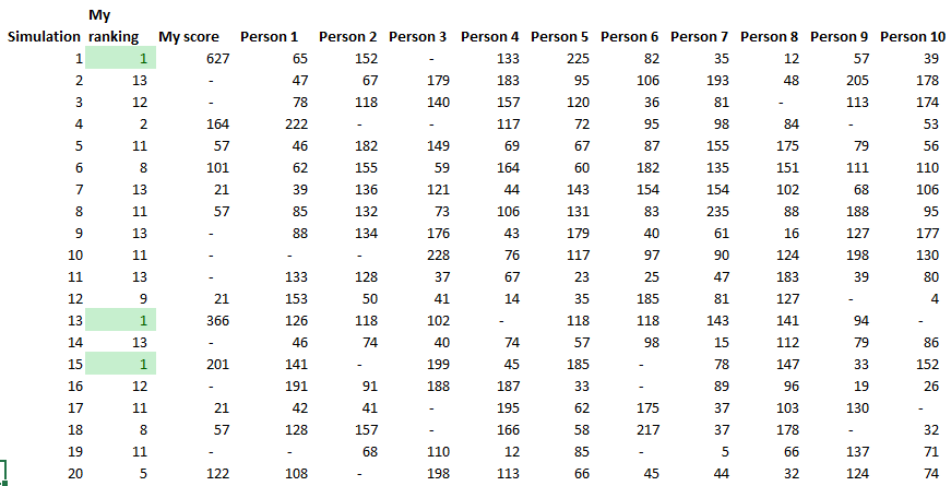 And we could then convert this into an EP table which would look like the following: 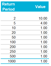 So we see that if we select these horses, we end up having somewhere between a 1 in 10 and a 1 in 5 chance of winning the competition. Now that we have all of this set up, we can then optimise our horse selection to target a particular return period. I didn’t actually end up setting up the above for the sweepstake, but I suspect it would have been an improvement on my approach Attempt 5 - Multiple day? There is a further refinement we can make to the above. We have so far only really been focusing on maximising our chance of winning by using a fixed strategy throughout the competition. But there is no reason we have to do this. After the first day, we should really be including the current scores of each competitor as part of our calculation of our ranking. i.e. if person 1 had a great day and now has 200 points but we had a bad day and still have 0 points, by accounting for this, the model should automatically increase our volatility i.e. start picking horses with longer odds so as to increase the chance of us catching up. If on the other hand, we had a really good first day and are now in the lead, the model should then automatically reduce our volatility and start selecting the favourites more often to help safely maintain our lead. How did it work in practice? I ended up placing 2nd, and taking 20% of the prize pot which was great! I was behind for most of the competition but then pulled back on the last day when a 66/1 came in 1st place, and I picked up 330 points off a single race. This may look miraculous, but is exactly how the model is supposed to work. Does that have any applicability to gambling generally? Unfortunately not, basically all of the work above is based on exploiting the specific scoring system of the sweepstake. There's no real way of apply this to gambling generally. Converting a Return Period to a RoL15/3/2019 I came across a useful way of looking at Rate on Lines last week, I was talking to a broker about what return periods to use in a model for various levels of airline market loss (USD250m, USD500m, etc.). The model was intended to be just a very high level, transparent market level model which we could use as a framework to discuss with an underwriter. We were talking through the reasonableness of the assumptions when the broker came out with the following: 'Well, you’d pay about 12.5 on line in the retro market at that attachment level, so that’s a 1 in 7 break-even right?' My response was: 'ummmm, come again?' His reasoning was as follows: Suppose the ILW pays $1$ @ $100$% reinstatements, and that it costs $12.5$% on line. Then if the layer suffers a loss, the insured will have a net position on the contract of $75$%. This is the $100$% limit which they receive due to the loss, minus the original $12.5$% Premium, minus an additional $12.5$% reinstatement Premium. The reinsurer will now need another $6$ years at $12.5$% RoL $(0.0125 * 6 = 0.75)$ to recover the limit and be at break-even. Here is a breakdown of the cashflow over the seven years for a $10m$ stretch at $12.5$% RoL: 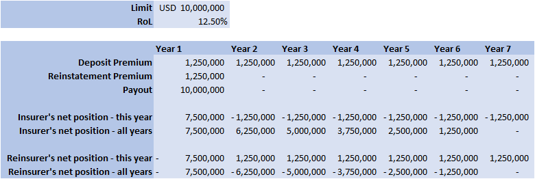 So the loss year plus the six clean years, tells us that if a loss occurs once every 7 years, then the contract is at break-even for this level of RoL.
So this is kind of cool - any time we have a RoL for a retro layer, we can immediately convert it to a Return Period for a loss which would trigger the layer. Generalisation 1 – various rates on line We can then generalise this reasoning to apply to a layer with an arbitrary RoL. Using the same reasoning as above, the break-even return period ends up being: $RP= 1 + \frac{(1-2*RoL)}{RoL}$ Inverting this gives: $RoL = \frac{1}{(1 + RP)}$ So let's say we have an ILW costing $7.5$% on line, the break-even return period is: $1 + \frac{(1-0.15)}{0.075} = 11.3$ Or let’s suppose we have a $1$ in $19$ return period, the RoL will be: $0.05 = \frac{1}{(1 + 19)}$ Generalisation 2 – other non-proportional layers The formula we derived above was originally intended to apply to ILWs, but it also holds any time we think the loss to the layer, if it occurs, will be a total loss. This might be the case for a cat layer, or a clash layers (layers which have an attachment above the underwriting limit for a single risk), or any layer with a relatively high attachment point compared to the underwriting limit. Adjustments to the formulas There are a few of adjustments we might need to make to these formulas before using them in practice. Firstly, the RoL above has no allowance for profit or expense loading, we can account for this by converting the market RoL to a technical RoL, this is done by simply dividing the RoL by $120-130$% (or any other appropriate profit/expense loading). This has the effect of increasing the number of years before the loss is expected to occur. Alternately, if layer does not have a paid reinstatement, or has a different factor than $100$%, then we would need to amend the multiple we are multiplying the RoL by in the formula above. For example, with nil paid reinstatements, the formula would be: $RP = 1 + \frac{(1-RoL)}{RoL}$ Another refinement we might wish to make would be to weaken the total loss assumption. We would then need to reduce the RoL by an appropriate amount to account for the possibility of partial losses. It’s going to be quite hard to say how much this should be adjusted for – the lower the layer the more it would need to be. Extending the Copula Method26/8/2018 If you have ever generated Random Variables stochastically using a Gaussian Copula, you may have noticed that the correlation of the generated sample ends up being lower than the value of the Covariance matrix of the underlying multivariate Gaussian Distribution. For an explanation of why this happens you can check out a previous post of mine: www.lewiswalsh.net/blog/correlations-friedrich-gauss-and-copula. It would be nice if we could amend our method to compensate for this drop. As a quick fix, we can simply run the model a few times and fudge the Covariance input until we get the desired Correlation value. If the model runs quickly, this is quite easy to do, but as soon as the model starts to get bigger and slower, it quickly becomes impractical to run it three of four times just to get the output Correlation we desire. We can do better than this. The insight we rely on is that for a Gaussian Copula, the Pearson Correlation in the generated sample just depends on the Covariance Value. We can therefore create a precomputed table of Input and Output values, and use this to select the correct input value for the desired output. I wrote some R code to do just that, we compute a table of Pearson's Correlations obtained for various Input Covariance values when using the Gaussian Copula.
a <- library(MASS)
library(psych)

set.seed(100)

m <- 2
n <- 10^6

OutputCor <- 0
InputCor <- 0

for (i in 1:100) {

  sigma <- matrix(c(1, i/100,
                    i/100, 1),
                  nrow=2)
  z <- mvrnorm(n,mu=rep(0, m),Sigma=sigma,empirical=T)

  u <- pnorm(z)

  OutputCor[i] <- cor(u,method='pearson')[1,2]
  InputCor[i] <- i/10

}

OutputCor
InputCor
Here is a sample from the table of results. You can see that the drop is relatively modest, but it does apply consistent across the whole table. 
Here is a graph showing the drop in values: 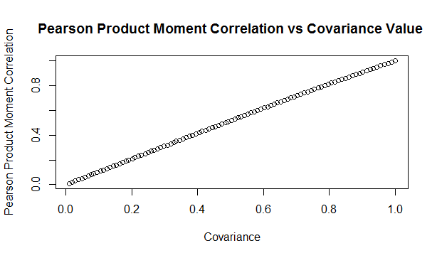
Updated Algorithm
We can then use the pre-computed table, interpolating where necessary, to give us a Covariance value for our Multivariate Gaussian Distribution which will generate the desired Pearson Product Moment Correlation Value. So for example, if we would like to generate a sample with a Pearson Product Moment value of $0.5$, according to our table, we would need to use $0.517602$ as an input Covariance. We can test these values using the following code:
a <- library(MASS)
library(psych)

set.seed(100)

m <- 2
n <- 5000000
sigma <- matrix(c(1, 0.517602,
                  0.517602, 1),
                nrow=2)
z <- mvrnorm(n,mu=rep(0, m),Sigma=sigma,empirical=T)
u <- pnorm(z)

cor(u,method='pearson')
Analytic Formulas I tried to find an analytic formula for the Product Moment values obtained in this manner, but I couldn't find anything online, and I also wasn't able to derive one myself. If we could find one, then instead of using the precompued table, we would be able to simply calculate the correct value. While searching, I did come across a number of interesting analytic formulas linking the values of Kendall's Tau, Spearman's Rank, and the input Covariance.. All the formulas below are from Fang, Fang, Kotz (2002) Link to paper: www.sciencedirect.com/science/article/pii/S0047259X01920172 The paper gives the following two results, where $\rho$ is the Pearson's Product Moment
$$\tau = \frac{2}{\pi} arcsin ( \rho ) $$ $$ {\rho}_s = \frac{6}{\pi} arcsin ( \frac{\rho}{2} ) $$
We can then use these formulas to extend our method above further to calculate an input Covariance to give any desired Kendall Tau, or Spearman's Rank. I initially thought that they would link the Pearson Product Moment value with Kendall or Spearman's measure, in which case we would still have to use the precomputed table. After testing it I realised that it is actually linking the Covariance to Kendall and Spearman's measures. Thinking about it, Kendall's Tau, and Spearman's Rank are both invariant to the reverse Gaussian transformation when moving from $z$ to $u$ in the algorithm. Therefore the problem of deriving an analytic formula for them is much simpler as one only has to link their values for a multivariate Gaussian Distribution. Pearson's however does change, therefore it is a completely different problem and may not even have a closed form solution. As an example of how to use the above formula, suppose we'd like our generated data to have a Kendall's Tau of $0.4$. First we need to invert the Kendall's Tau formula: $$ \rho = sin ( \frac{ \tau \pi }{2} ) $$ We then plug in $\rho = 0.4 $ giving:
$$ \rho = sin ( \frac{ o.4 \pi }{2} ) = 0.587785 $$
Giving usan input Covariance value of $0.587785$
We can then test this value with the following R code:
a <- library(MASS)
library(psych)

set.seed(100)

m <- 2
n <- 50000
sigma <- matrix(c(1, 0.587785,
                  0.587785, 1),
                nrow=2)
z <- mvrnorm(n,mu=rep(0, m),Sigma=sigma,empirical=T)
u <- pnorm(z)
cor(z,method='kendall')
Which we see gives us the value of $\tau$ we want. In this case the difference between the input Covariance $0.587785$, and the value of Kendall's Tau $0.4$ is actually quite significant. It's the second week of your new job Capital Modelling job. After days spent sorting IT issues, getting lost coming back from the toilets, and perfecting your new commute to work (probability of getting a seat + probability of delay * average journey temperature.) your boss has finally given you your first real project to work on. You've been asked to carry out an annual update of the Underwriting Risk Capital Charge for a minor part of the company's Motor book. Not the grandest of analysis you'll admit, this particular class only makes up about 0.2% of the company's Gross Written Premium, and the Actuaries who reserve the company's bigger classes would probably consider the number of decimal places used in the annual report more material than your entire analysis. But you know in your heart of hearts that this is just another stepping stone on your inevitable meteoric rise to Chief Actuary in the Merger and Acquisition department, where one day you will pass judgement on billion dollar deals in-between expensive lunches with CFOs, and drinks with journalists on glamorous rooftop bars. The company uses in-house reserving software, but since you're not that familiar with it, and because you want to make a good impression, you decide to carry out extensive checking of the results in Excel. You fire up the Capital Modelling Software (which may or may not have a name that means a house made out of ice), put in your headphones and grind it out. Hours later you emerge triumphant, and you've really nailed it, your choice of correlation (0.4), and correlation method (Gaussian Copula) is perfect. As planned you run extracts of all the outputs, and go about checking them in Excel. But what's this? You set the correlation to be 0.4 in the software, but when you check the correlation yourself in Excel, it's only coming out at 0.384?! What's going on? Simulating using Copulas The above is basically what happened to me (minus most of the actual details. but I did set up some modelling with correlated random variables and then checked it myself in Excel and was surprised to find that the actual correlation in the generated output was always lower than the input.) I looked online but couldn't find anything explaining this phenomenon, so I did some investigating myself. So just to restate the problem, when using Monte Carlo simulation, and generating correlated random variables using the Copula method. When we actually check the correlation of the generated sample, it always has a lower correlation than the correlation we specified when setting up the modelling. My first thought for why this was happening was that were we not running enough simulations and that the correlations would eventually converge if we just jacked up the number of simulations. This is the kind of behaviour you see when using Monte Carlo simulation and not getting the mean or standard deviation expected from the sample. If you just churn through more simulations, your output will eventually converge. When creating Copulas using the Gaussian Method, this is not the case though, and we can test this. I generated the graph below in R to show the actual correlation we get when generating correlated random variables using the Copula method for a range of different numbers of simulations. There does seem to be some sort of loose limiting behaviour, as the number of simulations increases, but the limit appears to be around 0.384 rather than 0.4. 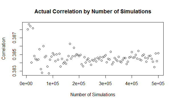
The actual explanation First, we need to briefly review the algorithm for generating random variables with a given correlation using the normal copula. Step 1 - Simulate from a multivariate normal distribution with the given covariance matrix. Step 2 - Apply an inverse gaussian transformation to generate random variables with marginal uniform distribution, but which still maintain a dependency structure Step 3 - Apply the marginal distributions we want to the random variables generated in step 2 We can work through these three steps ourselves, and check at each step what the correlation is. The first step is to generate a sample from the multivariate normal. I'll use a correlation of 0.4 though out this example. Here is the R code to generate the sample:
a <- library(MASS)
library(psych)
set.seed(100)
m <- 2
n <- 1000
sigma <- matrix(c(1, 0.4,
0.4, 1),
nrow=2)
z <- mvrnorm(n,mu=rep(0, m),Sigma=sigma,empirical=T)
And here is a Scatterplot of the generated sample from the multivariate normal distribution: 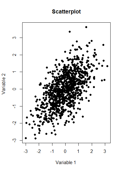
We now want to check the product moment correlation of our sample, which we can do using the following code: cor(z,method='pearson') Which gives us the following result: > cor(z,method='pearson') [,1] [,2] [1,] 1.0 0.4 [2,] 0.4 1.0 So we see that the correlation is 0.4 as expected. The Psych package has a useful function which produces a summary showing a Scatterplot, the two marginal distribution, and the correlation: 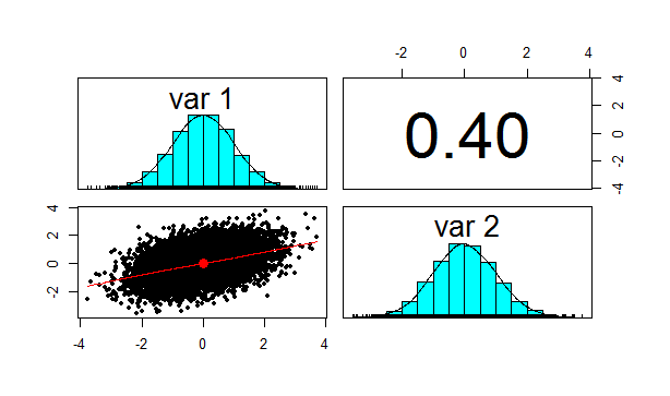
Let us also check Kendall's Tau and Spearman's rank at this point. This will be instructive later on. We can do this using the following code: cor(z,method='spearman') cor(z,method='Kendall') Which gives us the following results: > cor(z,method='spearman') [,1] [,2] [1,] 1.0000000 0.3787886 [2,] 0.3787886 1.0000000 > cor(z,method='kendall') [,1] [,2] [1,] 1.0000000 0.2588952 [2,] 0.2588952 1.0000000 Note that this is less than 0.4 as well, but we will discuss this further later on.
We now need to apply step 2 of the algorithm, which is applying the inverse Gaussian transformation to our multivariate normal distribution. We can do this using the following code:
u <- pnorm(z) We now want to check the correlation again, which we can do using the following code: cor(z,method='spearman') Which gives the following result: > cor(z,method='spearman') [,1] [,2] [1,] 1.0000000 0.3787886 [2,] 0.3787886 1.0000000 Here is the Psych summary again: 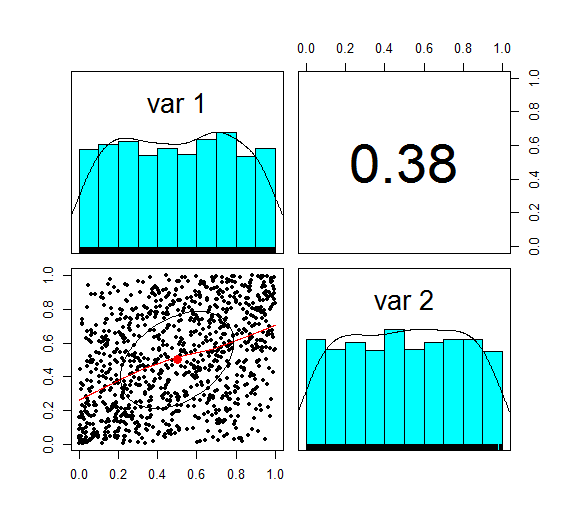
u is now marginally uniform (hence the name). We can see this by looking at the Scatterplot and marginal pdfs above. We also see that the correlation has dropped to 0.379, down from 0.4 at step 1. The Pearson correlation measures the linear correlation between two random variables. We generated normal random variables, which had the required correlation, but then we applied a non-linear (inverse Gaussian) transformation. This non-linear step is the source of the dropped correlation in our algorithm. We can also retest Kendall's Tau, and Spearman's at this point using the following code: cor(z,method='spearman') cor(z,method='Kendall') This gives us the following result: > cor(u,method='spearman') [,1] [,2] [1,] 1.0000000 0.3781471 [2,] 0.3781471 1.0000000 > cor(u,method='kendall') [,1] [,2] [1,] 1.0000000 0.2587187 [2,] 0.2587187 1.0000000 Interestingly, these values have not changed from above! i.e. we have preserved these measures of correlation between step 1 and step 2. It's only the Pearson correlation measure (which is a measure of linear correlation) which has not been preserved. Let's now apply the step 3, and once again retest our three correlations. The code to carry out step 3 is below: x1 <- qgamma(u[,1],shape=2,scale=1) x2 <- qbeta(u[,2],2,2) df <- cbind(x1,x2) pairs.panels(df) The summary for step 3 looks like the following. 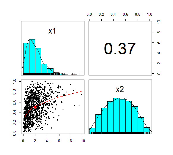
This is the end goal of our method. We see that our two marginal distributions have the required distribution, and we have a correlation between them of 0.37. Let's recheck our three measures of correlation. cor(df,method='pearson') cor(df,meth='spearman') cor(df,method='kendall') > cor(df,method='pearson') x1 x2 x1 1.0000000 0.3666192 x2 0.3666192 1.0000000 > cor(df,meth='spearman') x1 x2 x1 1.0000000 0.3781471 x2 0.3781471 1.0000000 > cor(df,method='kendall') x1 x2 x1 1.0000000 0.2587187 x2 0.2587187 1.0000000 So the Pearson has reduced again at this step, but the Spearman and Kendall's Tau are once again the same.
Does this matter?
This does matter, let's suppose you are carrying out capital modelling and using this method to correlate your risk sources. Then you would be underestimating the correlation between random variables, and therefore potentially underestimating the risk you are modelling. Is this just because we are using a Gaussian Copula? No, this is the case for all Copulas. Is there anything you can do about it? Yes, one solution is to just increase the input correlation by a small amount, until we get the output we want. A more elegant solution would be to build this scaling into the method. The amount of correlation lost at the second step is dependent just on the input value selected, so we could pre-compute a table of input and output correlations, and then based on the desired output, we would be able to look up the exact input value to use. If you have played around with Correlating Random Variables using a Correlation Matrix in [insert your favourite financial modelling software] then you may have noticed the requirement that the Correlation Matrix be positive semi-definite. But what exactly does this mean? And how would we check this ourselves in VBA or R? Mathematical Definition Let's start with the Mathematical definition. To be honest, it didn't really help me much in understanding what's going on, but it's still useful to know.
A symmetric $n$ x $n$ matrix $M$ is said to be positive semidefinite if the scalar $z^T M z $ is positive for every non-zero column vector $z$ of $n$ real numbers.
If I am remembering my first year Linear Algebra course correctly, then Matrices can be thought of as transformations on Vector Spaces. Here the Vector Space would be a collection of Random Variables. I'm sure there's some clever way in which this gives us some kind of non-degenerate behaviour. After a bit of research online I couldn't really find much. Intuitive Definition The intuitive explanation is much easier to understand. The requirement comes down to the need for internal consistency between the correlations of the Random Variables. For example, suppose we have three Random Variables, A, B, C. Let's suppose that A and B are highly correlated, that is to say, when A is a high value, B is also likely to be a high value. Let's also suppose that A and C are highly correlated, so that if A is a high value, then C is also likely to be a high value. We have now implicitly defined a constraint on the correlation between B and C. If A is high both B and C are also high, so it can't be the case that B and C are negatively correlated, i.e. that when B is high, C is low. Therefore some correlation matrices will give relations which are impossible to model. Alternative characterisations You can find a number of necessary and sufficient conditions for a matrix to be positive definite, I've included some of them below. I used number 2 in the VBA code for a real model I set up to check for positive definiteness. 1. All Eigenvalues are positive. If you have studied some Linear Algebra, then you may not be surprised to learn that there is a characterization using Eigenvalues. It seems like just about anything to do with Matrices can be restated in terms of Eigenvalues. I'm not really sure how to interpret this condition though in an intuitive way. 2. All leading principal minors are all positive This is the method I used to code the VBA algorithm below. The principal minors are just another name for the determinant of the upper-left $k$ by $k$ sub-matrix. Since VBA has a built in method for returning the determinant of a matrix this was quite an easy method to code. 3. It has a unique Cholesky decomposition I don't really understand this one properly, however I remember reading that Cholesky decomposition is used in the Copula Method when sampling Random Variables, therefore I suspect that this characterisation may be important! Since I couldn't really write much about Cholesky decomposition here is a picture of Cholesky instead, looking quite dapper. 
All 2x2 matrices are positive semi-definite Since we are dealing with Correlation Matrices, rather than arbitrary Matrices, we can actually show a-priori that all 2 x 2 Matrices are positive semi-definite. Proof
Let M be a $2$ x $2$ correlation matrix.
$$M = \begin{bmatrix} 1&a\\ a&1 \end{bmatrix}$$ And let $z$ be the column vector $M = \begin{bmatrix} z_1\\ z_2 \end{bmatrix}$ Then we can calculate $z^T M z$ $$z^T M z = {\begin{bmatrix} z_1\\ z_2 \end{bmatrix}}^T \begin{bmatrix} 1&a\\ a&1 \end{bmatrix} \begin{bmatrix} z_1\\ z_2 \end{bmatrix} $$ Multiplying this out gives us: $$ = {\begin{bmatrix} z_1\\ z_2 \end{bmatrix}}^T \begin{bmatrix} z_1 & a z_2 \\ a z_1 & z_2 \end{bmatrix} = z_1 (z_1 + a z_2) + z_2 (a z_1 + z_2)$$ We can then simplify this to get: $$ = {z_1}^2 + a z_1 z_2 + a z_1 z_2 + {z_2}^2 = (z_1 + a z_2)^2 \geq 0$$ Which gives us the required result. This result is consistent with our intuitive explanation above, we need our Correlation Matrix to be positive semidefinite so that the correlations between any three random variables are internally consistent. Obviously, if we only have two random variables, then this is trivially true, so we can define any correlation between two random variables that we like. Not all 3x3 matrices are positive semi-definite The 3x3 case, is simple enough that we can derive explicit conditions. We do this using the second characterisation, that all principal minors must be greater than or equal to 0.
Demonstration
Let M be a $3$ x $3$ correlation matrix: $$M = \begin{bmatrix} 1&a&b\\ a&1&c \\ b&c&1 \end{bmatrix}$$ We first check the determinant of the $2$ x $2$ sub matrix. We need that: $ \begin{vmatrix} 1 & a \\ a & 1 \end{vmatrix} \geq 0 $ By definition: $ \begin{vmatrix} 1 & a \\ a & 1 \end{vmatrix} = 1 - a^2$ We have that $ | a | \leq 1 $, hence $ | a^2 | \leq 1 $, and therefore: $ | 1- a^2 | \geq 0 $ Therefore the determinant of the $2$ x $2$ principal sub-matrix is always positive. Now to check the full $3$ x $3$. We require: $ \begin{vmatrix} 1 & a & b \\ a & 1 & c \\ b & c & 1 \end{vmatrix} \geq 0 $ By definition: $ \begin{vmatrix} 1 & a & b \\ a & 1 & c \\ b & c & 1 \end{vmatrix} = 1 ( 1 - c^2) - a (a - bc) + b(ac - b) = 1 + 2abc - a^2 - b^2 - c^2 $ Therefore in order for a $3$ x $3$ matrix to be positive demi-definite we require: $a^2 + b^2 + c^2 - 2abc = 1 $ I created a 3d plot in R of this condition over the range [0,1]. 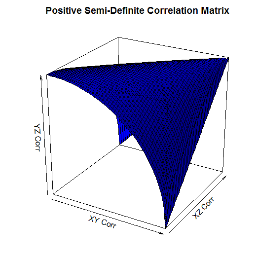
It's a little hard to see, but the way to read this graph is that the YZ Correlation can take any value below the surface. So for example, when the XY Corr is 1, and the XZ Corr is 0, the YZ Corr has to be 0. When the XY Corr is 0 on the other hand, and XZ Corr is also 0, then the YZ Corr can be any value between 0 and 1. Checking that a Matrix is positive semi-definite using VBA When I needed to code a check for positive-definiteness in VBA I couldn't find anything online, so I had to write my own code. It makes use of the excel determinant function, and the second characterization mentioned above. Note that we only need to start with the 3x3 sub matrix as we know from above that all 1x1 and all 2x2 determinants are positive. This is not a very efficient algorithm, but it works and it's quite easy to follow.
Function CheckCorrMatrixPositiveDefinite()
Dim vMatrixRange As Variant
Dim vSubMatrix As Variant
Dim iSubMatrixSize As Integer
Dim iRow As Integer
Dim iCol As Integer
Dim bIsPositiveDefinite As Boolean
bIsPositiveDefinite = True
vMatrixRange = Range(Range("StartCorr"), Range("StartCorr").Offset(inumberofrisksources - 1, inumberofrisksources - 1))
' Only need to check matrices greater than size 2 as determinant always greater than 0 when less than or equal to size 2'
If iNumberOfRiskSources > 2 Then
For iSubMatrixSize = iNumberOfRiskSources To 3 Step -1
ReDim vSubMatrix(iSubMatrixSize - 1, iSubMatrixSize - 1)
For iRow = 1 To iSubMatrixSize
For iCol = 1 To iSubMatrixSize
vSubMatrix(iRow - 1, iCol - 1) = vMatrixRange(iRow, iCol)
Next
Next
'If the determinant of the matrix is 0, then the matrix is semi-positive definite'
If Application.WorksheetFunction.MDeterm(vSubMatrix) < 0 Then
CheckCorrMatrixisPositiveDefinite = False
bIsPositiveDefinite = False
End If
Next
End If
If bIsPositiveDefinite = True Then
CheckCorrMatrixPositiveDefinite = True
Else
CheckCorrMatrixPositiveDefinite = False
End If
End Function
Checking that a Matrix is positive semi-definite in R Let's suppose that instead of VBA you were using an actually user friendly language like R. What does the code look like then to check that a matrix is positive semi-definite? All we need to do is install a package called 'Matrixcalc', and then we can use the following code: is.positive.definite( Matrix ) That's right, we needed to code up our own algorithm in VBA, whereas with R we can do the whole thing in one line using a built in function! It goes to show that the choice of language can massively effect how easy a task is. |
AuthorI work as an actuary and underwriter at a global reinsurer in London. Categories
All
Archives
April 2024
|
 RSS Feed