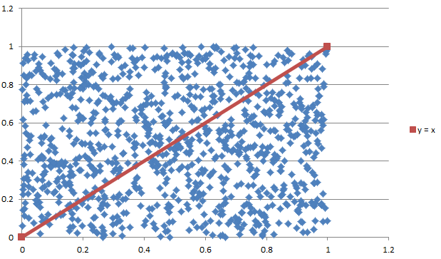
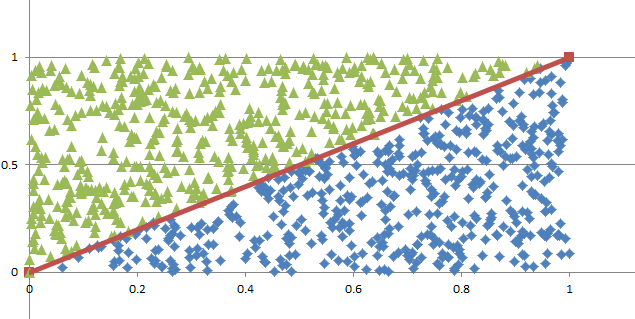
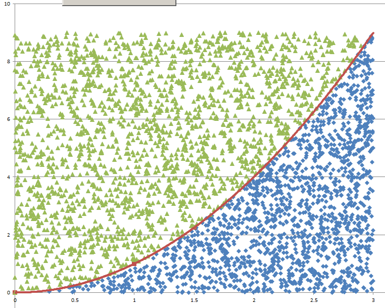
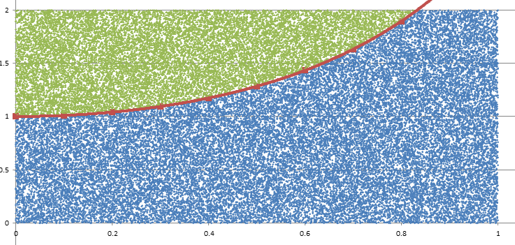
Monte Carlo Integration

I blogged a while ago about using Monte Carlo methods to estimate the value of $\pi$.

We used random sampling inside a unit square and then counted the proportion of sample points that landed inside a unit circle. We knew what the area of the unit circle was - $\pi$ - and we could therefore relate the area we had calculated using random sampling with the known area of the circle.

It got my thinking that there is actually another way to think about what we did - we numerically integrated the unit circle and then compared this to the known value of the integral using analytical methods. But why can't we use this method to numerically integrate other shapes and curves? It turns out we can!

Lets set up some problems and look at how it works in practice.

Problem 1 - y = x

Integrate y = x from x = 0 to x = 1.

I first sampled 1000 points in the unit square and put them in a chart along with the line we are trying to integrate. This is just to help visualise what we are trying to do.

​Since we are interested in the area under the curve I coloured all these points in a different colour.

Since we have sampled randomly from the square, we would expect the proportion of points falling below the line will approach the proportion of the area below and above the line.

If we examine this ratio we get a value of $ 492 / 1000 $ which is very close to the value of $1/2$ we would expect from analytical methods.

Problem 2 - y = x ^ 2

Let's try again on a harder problem. What is the integral of $y = x^2$ between $0$ and $3$?

Let's create another graph of this problem:
​

When we look at the results we see that the ratio now is 0.3326, which once again we can see is converging to the answer we expect of 0.3333.

I had to bump the number of simulations up to 5000 in this example to get a reasonable fit.

​Problem 3 - e^(x^2)

You might be thinking to yourself at this point - all this is quite interesting but is there any benefit it doing things this way? All we've done so far is check the solutions to intergrals that we already know how to solve!

The integral for this problem however is known to have no elementary closed solution. That means that we can't just use A-level maths to calculate the integral.

The graph of the function isn't too complicated and looks like this:

I had to bump up the number of simulations here again to 50,000, but the analysis gave us a figure of 1.46 for the value of the integral.

So why does this particular problem matter again? It means that this method is not just an interesting curiosity. But that it actually allows solutions to be calculated for integrals which standard A-level integration techniques don't work for.