Converting a Return Period to a RoL

I came across a useful way of looking at Rate on Lines last week, I was talking to a broker about what return periods to use in a model for various levels of airline market loss (USD250m, USD500m, etc.). The model was intended to be just a very high level, transparent market level model which we could use as a framework to discuss with an underwriter. We were talking through the reasonableness of the assumptions when the broker came out with the following:
 
'Well, you’d pay about 12.5 on line in the retro market at that attachment level, so that’s a 1 in 7 break-even right?'
 
My response was:

'ummmm, come again?'
 
His reasoning was as follows:
 
Suppose the ILW pays $1$ @ $100$% reinstatements, and that it costs $12.5$​% on line.
Then if the layer suffers a loss, the insured will have a net position on the contract of $75$%. This is the $100$% limit which they receive due to the loss, minus the original $12.5$% Premium, minus an additional $12.5$% reinstatement Premium. The reinsurer will now need another $6$ years at $12.5$% RoL $(0.0125 * 6 = 0.75)$ to recover the limit and be at break-even.
 
Here is a breakdown of the cashflow over the seven years for a $10m$ stretch at $12.5$% RoL: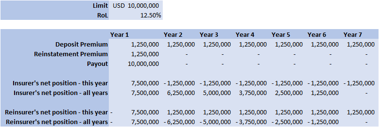
 

So the loss year plus the six clean years, tells us that if a loss occurs once every 7 years, then the contract is at break-even for this level of RoL.

So this is kind of cool - any time we have a RoL for a retro layer, we can immediately convert it to a Return Period for a loss which would trigger the layer.
 
Generalisation 1 – various rates on line
 
We can then generalise this reasoning to apply to a layer with an arbitrary RoL. Using the same reasoning as above, the break-even return period ends up being:
 
$RP= 1 + \frac{(1-2*RoL)}{RoL}$
 
Inverting this gives:
 
$RoL = \frac{1}{(1 + RP)}$
 
So let's say we have an ILW costing $7.5$% on line, the break-even return period is:
 
$1 + \frac{(1-0.15)}{0.075} = 11.3$
 
Or let’s suppose we have a $1$ in $19$ return period, the RoL will be:
 
$0.05 = \frac{1}{(1 + 19)}$
 
Generalisation 2 – other non-proportional layers
 
The formula we derived above was originally intended to apply to ILWs, but it also holds any time we think the loss to the layer, if it occurs, will be a total loss. This might be the case for a cat layer, or a clash layers (layers which have an attachment above the underwriting limit for a single risk), or any layer with a relatively high attachment point compared to the underwriting limit.
 
Adjustments to the formulas
 
There are a few of adjustments we might need to make to these formulas before using them in practice.
 
Firstly, the RoL above has no allowance for profit or expense loading, we can account for this by converting the market RoL to a technical RoL, this is done by simply dividing the RoL by $120-130$% (or any other appropriate profit/expense loading). This has the effect of increasing the number of years before the loss is expected to occur.
 
Alternately, if layer does not have a paid reinstatement, or has a different factor than $100$%, then we would need to amend the multiple we are multiplying the RoL by in the formula above. For example, with nil paid reinstatements, the formula would be:
 
$RP = 1 + \frac{(1-RoL)}{RoL}$
 
Another refinement we might wish to make would be to weaken the total loss assumption.  We would then need to reduce the RoL by an appropriate amount to account for the possibility of partial losses. It’s going to be quite hard to say how much this should be adjusted for – the lower the layer the more it would need to be.