Poisson Distribution for small Lambda23/4/2019
I was asked an interesting question a couple of weeks ago when talking through some modelling with a client.
We were modelling an airline account, and for various reasons we had decided to base our large loss modelling on a very basic top-down allocation method. We would take a view of the market losses at a few different return periods, and then using a scenario approach, would allocate losses to our client proportionately. Using this method, the frequency of losses is then scaled down by the % of major policies written, and the severity of losses is scaled down by the average line size. To give some concrete numbers (which I’ve made up as I probably shouldn’t go into exactly what the client’s numbers were), let's say the company was planning on taking a line on around 10% of the Major Airline Risks, and their average line was around 1%. We came up with a table of return periods for market level losses. The table looked something like following (the actual one was also different to the table below, but not miles off): 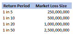
Then applying the 10% hit factor if there is a loss, and the 1% line written, we get the following table of return periods for our client:
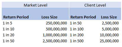
Hopefully all quite straightforward so far. As an aside, it is quite interesting to sometimes pare back all the assumptions to come up with something transparent and simple like the above. For airline risks, the largest single policy limit is around USD 2.5bn, so we are saying our worst case scenario is a single full limit loss, and that each year this has around a 1 in 50 chance of occurring. We can then directly translate that into an expected loss, in this case it equates to 50m (i.e. 2.5bn *0.02) of pure loss cost. If we don't think the market is paying this level of premium for this type of risk, then we better have a good reason for why we are writing the policy!
So all of this is interesting (I hope), but what was the original question the client asked me? We can see from the chart that for the market level the highest return period we have listed is 1 in 50. Clearly this does translate to a much longer return period at the client level, but in the meeting where I was asked the original question, we were just talking about the market level. The client was interested in what the 1 in 200 at the market level was and what was driving this in the modelling. The way I had structured the model was to use four separate risk sources, each with a Poisson frequency (lambda set to be equal to the relevant return period), and a fixed severity. So what this question translates to is, for small Lambdas $(<<1)$, what is the probability that $n=2$, $n=3$, etc.? And at what return period is the $n=2$ driving the $1$ in $200$? Let’s start with the definition of the Poisson distribution: Let $N \sim Poi(\lambda)$, then: $$P(N=n) = e^{-\lambda} \frac{ \lambda ^ n}{ n !} $$ We are interested in small $\lambda$ – note that for large $\lambda$ we can use a different approach and apply sterling’s approximation instead. Which if you are interested, I’ve written about here: www.lewiswalsh.net/blog/poisson-distribution-what-is-the-probability-the-distribution-is-equal-to-the-mean
For small lambda, the insight is to use a Taylor expansion of the $e^{-\lambda}$ term. The Taylor expansion of $e^{-\lambda}$ is:
$$ e^{-\lambda} = \sum_{i=0}^{\infty} \frac{\lambda^i}{ i!} = 1 - \lambda + \frac{\lambda^2}{2} + o(\lambda^2) $$
We can then examine the pdf of the Poisson distribution using this approximation: $$P(N=1) =\lambda e^{-\lambda} = \lambda ( 1 – \lambda + \frac{\lambda^2}{2} + o(\lambda^2) ) = \lambda - \lambda^2 +o(\lambda^2)$$
as in our example above, we have:
$$ P(N=1) ≈ \frac{1}{50} – {\frac{1}{50}}^2$$
This means that, for small lambda, the probability that $N$ is equal to $1$ is always slightly less than lambda. Now taking the case $N=2$: $$P(N=2) = \frac{\lambda^2}{2} e^{-\lambda} = \frac{\lambda^2}{2} (1 – \lambda +\frac{\lambda^2}{2} + o(\lambda^2)) = \frac{\lambda^2}{2} -\frac{\lambda^3}{2} +\frac{\lambda^4}{2} + o(\lambda^2) = \frac{\lambda^2}{2} + o(\lambda^2)$$
So once again, for $\lambda =\frac{ 1}{50}$ we have:
$$P(N=2) ≈ 1/50 ^ 2 /2 = P(N=1) * \lambda / 2$$
In this case, for our ‘1 in 50’ sized loss, we would expect to have two such losses in a year once every 5000 years! So this is definitely not driving our 1 in 200 result.
We can add some extra columns to our market level return periods as follows: 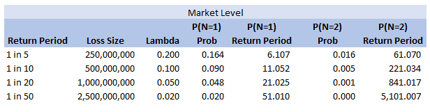
So we see for the assumptions we made, around the 1 in 200 level our losses are still primarily being driven by the P(N=1) of the 2.5bn loss, but then in addition we will have some losses coming through corresponding to P(N=2) and P(N=3) of the 250m and 500m level, and also combinations of the other return periods.
So is this the answer I gave to the client in the meeting? …. Kinda, I waffled on a bit about this kind of thing, but then it was only after getting back to the office that I thought about trying to breakdown analytically which loss levels we can expect to kick in at various return periods. Of course all of the above is nice but there is an easier way to see the answer, since we’d already stochastically generated a YLT based on these assumptions, we could have just looked at our YLT, sorted by loss size and then gone to the 99.5 percentile and see what sort of losses make up that level. The above analysis would have been more complicated if we have also varied the loss size stochastically. You would normally do this for all but the most basic analysis. The reason we didn’t in this case was so as to keep the model as simple and transparent as possible. If we had varied the loss size stochastically then the 1 in 200 would have been made up of frequency picks of various return periods, combined with severity picks of various return periods. We would have had to arbitrarily fix one in order to say anything interesting about the other one, which would not have been as interesting. |
AuthorI work as an actuary and underwriter at a global reinsurer in London. Categories
All
Archives
April 2024
|
 RSS Feed