Extending the Copula Method26/8/2018 If you have ever generated Random Variables stochastically using a Gaussian Copula, you may have noticed that the correlation of the generated sample ends up being lower than the value of the Covariance matrix of the underlying multivariate Gaussian Distribution. For an explanation of why this happens you can check out a previous post of mine: www.lewiswalsh.net/blog/correlations-friedrich-gauss-and-copula. It would be nice if we could amend our method to compensate for this drop. As a quick fix, we can simply run the model a few times and fudge the Covariance input until we get the desired Correlation value. If the model runs quickly, this is quite easy to do, but as soon as the model starts to get bigger and slower, it quickly becomes impractical to run it three of four times just to get the output Correlation we desire. We can do better than this. The insight we rely on is that for a Gaussian Copula, the Pearson Correlation in the generated sample just depends on the Covariance Value. We can therefore create a precomputed table of Input and Output values, and use this to select the correct input value for the desired output. I wrote some R code to do just that, we compute a table of Pearson's Correlations obtained for various Input Covariance values when using the Gaussian Copula.
a <- library(MASS)
library(psych)

set.seed(100)

m <- 2
n <- 10^6

OutputCor <- 0
InputCor <- 0

for (i in 1:100) {

  sigma <- matrix(c(1, i/100,
                    i/100, 1),
                  nrow=2)
  z <- mvrnorm(n,mu=rep(0, m),Sigma=sigma,empirical=T)

  u <- pnorm(z)

  OutputCor[i] <- cor(u,method='pearson')[1,2]
  InputCor[i] <- i/10

}

OutputCor
InputCor
Here is a sample from the table of results. You can see that the drop is relatively modest, but it does apply consistent across the whole table. 
Here is a graph showing the drop in values: 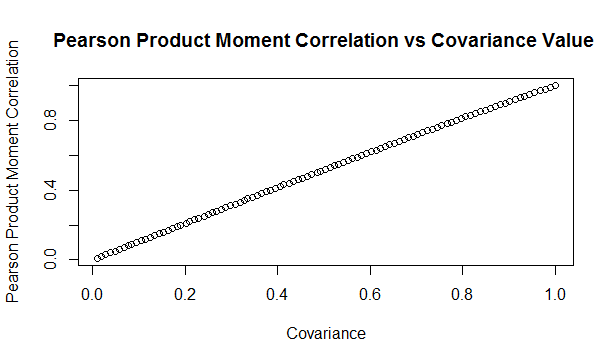
Updated Algorithm
We can then use the pre-computed table, interpolating where necessary, to give us a Covariance value for our Multivariate Gaussian Distribution which will generate the desired Pearson Product Moment Correlation Value. So for example, if we would like to generate a sample with a Pearson Product Moment value of $0.5$, according to our table, we would need to use $0.517602$ as an input Covariance. We can test these values using the following code:
a <- library(MASS)
library(psych)

set.seed(100)

m <- 2
n <- 5000000
sigma <- matrix(c(1, 0.517602,
                  0.517602, 1),
                nrow=2)
z <- mvrnorm(n,mu=rep(0, m),Sigma=sigma,empirical=T)
u <- pnorm(z)

cor(u,method='pearson')
Analytic Formulas I tried to find an analytic formula for the Product Moment values obtained in this manner, but I couldn't find anything online, and I also wasn't able to derive one myself. If we could find one, then instead of using the precompued table, we would be able to simply calculate the correct value. While searching, I did come across a number of interesting analytic formulas linking the values of Kendall's Tau, Spearman's Rank, and the input Covariance.. All the formulas below are from Fang, Fang, Kotz (2002) Link to paper: www.sciencedirect.com/science/article/pii/S0047259X01920172 The paper gives the following two results, where $\rho$ is the Pearson's Product Moment
$$\tau = \frac{2}{\pi} arcsin ( \rho ) $$ $$ {\rho}_s = \frac{6}{\pi} arcsin ( \frac{\rho}{2} ) $$
We can then use these formulas to extend our method above further to calculate an input Covariance to give any desired Kendall Tau, or Spearman's Rank. I initially thought that they would link the Pearson Product Moment value with Kendall or Spearman's measure, in which case we would still have to use the precomputed table. After testing it I realised that it is actually linking the Covariance to Kendall and Spearman's measures. Thinking about it, Kendall's Tau, and Spearman's Rank are both invariant to the reverse Gaussian transformation when moving from $z$ to $u$ in the algorithm. Therefore the problem of deriving an analytic formula for them is much simpler as one only has to link their values for a multivariate Gaussian Distribution. Pearson's however does change, therefore it is a completely different problem and may not even have a closed form solution. As an example of how to use the above formula, suppose we'd like our generated data to have a Kendall's Tau of $0.4$. First we need to invert the Kendall's Tau formula: $$ \rho = sin ( \frac{ \tau \pi }{2} ) $$ We then plug in $\rho = 0.4 $ giving:
$$ \rho = sin ( \frac{ o.4 \pi }{2} ) = 0.587785 $$
Giving usan input Covariance value of $0.587785$
We can then test this value with the following R code:
a <- library(MASS)
library(psych)

set.seed(100)

m <- 2
n <- 50000
sigma <- matrix(c(1, 0.587785,
                  0.587785, 1),
                nrow=2)
z <- mvrnorm(n,mu=rep(0, m),Sigma=sigma,empirical=T)
u <- pnorm(z)
cor(z,method='kendall')
Which we see gives us the value of $\tau$ we want. In this case the difference between the input Covariance $0.587785$, and the value of Kendall's Tau $0.4$ is actually quite significant. |
AuthorI work as an actuary and underwriter at a global reinsurer in London. Categories
All
Archives
April 2024
|
 RSS Feed