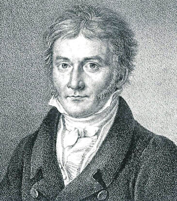
I noticed something surprising about the Maximum Likelihood Estimator (MLE) for a uniform distribution yesterday.

Suppose we’re given sample $X’ = {x_1, x_2, … x_n}$ from a uniform distribution $X$ with parameters $a,b$. Then the MLE estimator for $a = min(X’)$, and $b = max(X’)$. [1] All straight forward so far.

However, examining the estimators, we can also say with probability = 1 that $a < min(X’)$, and similarly that $b > max(X’)$. Isn't it strange that the MLE estimators are clearly less/more than the true values? 

So what can we do instead?

Let me introduce a game – I keep flipping a coin and you have to guess whether it will come up heads or tails. The prize pot starts at \$2, and each time you guess correctly the prize pot doubles, we keep playing until you eventually guess incorrectly at which point you get whatever has accumulated in the prize pot.

So if you guess wrong on the first flip, you just get the \$2. If you guess wrong on the second flip you get \$4, and if you get it wrong on the 10th flip you get \$1024.

Knowing this, how much would you pay to enter this game?

You're guaranteed to win at least \$2, so you'd obviously pay at least $\2. There is a 50% chance you'll win \$4, a 25% chance you'll win \$8, a 12.5% chance you'll win \$16, and so on. Knowing this maybe you'd pay \$5 to play - you'll probably lose money but there's a decent chance you'll make quite a bit more than \$5.
​
Perhaps you take a more mathematical approach than this. You might reason as follows – ‘I’m a rational person therefore as any good rational person should, I will calculate the expected value of playing the game, this is the maximum I should be willing to play the game’. This however is the crux of the problem and the source of the paradox, most people do not really value the game that highly – when asked they’d pay somewhere between \$2-\$10 to play it, and yet the expected value of the game is infinite.... 

Source: https://unsplash.com/@pujalin

​The above is a lovely photo I found of St Petersburg. The reason the paradox is named after St Petersburg actually has nothing to do with the game itself, but is due to an early article published by Daniel Bernoulli in a St Petersburg journal. As an aside, having just finished the book A Gentleman in Moscow by Amor Towles (which I loved and would thoroughly recommend) I'm curious to visit Moscow and St Petersburg one day.
​

I'm always begrudgingly impressed by brokers and underwriters who can do most of their job without resorting to computers or a calculator. If you give them a gross premium for a layer, they can reel off gross and net rates on line, the implied loss cost, and give you an estimate of the price for a higher layer using an ILF in their head. When I'm working, so much actuarial modelling requires a computer (sampling from probability distributions, Monte Carlo methods, etc.) that just to give any answer at all I need to fire up Excel and make a Spreadsheet. So anytime there's a chance to do some shortcuts I'm always all for it!

One mental calculation trick which is quite useful when working with compound interest is called the Rule of 72. It states that for interest rate $i$, under growth from annual compound interest, it takes approximately $\frac{72}{i} $ years for a given value to double in size.

Why does it work?

Here is a quick derivation showing why this works, all we need is to manipulate the exact solution with logarithms and then play around with the Taylor expansion.

We are interested in the following identity, which gives the exact value of $n$ for which an investment doubles under compound interest:
$$ \left( 1 + \frac{i}{100} \right)^n = 2$$
Taking logs of both sides gives the following:
$$ ln \left( 1 + \frac{i}{100} \right)^n = ln(2)$$
And then bringing down the $n$:
$$n* ln \left( 1 + \frac{i}{100} \right) = ln(2)$$
And finally solving for $n$:
$$n = \frac {ln(2)} { ln \left( 1 + \frac{i}{100} \right) }$$
So the above gives us a formula for $n$, the number of years. We now need to come up with a simple approximation to this function, and we do so by examining the Taylor expansion denominator of the right have side:

We can compute the value of $ln(2)$:

The Taylor expansion of the denominator is:
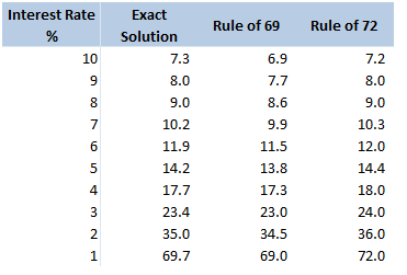
$$ln \left( 1 + \frac{i}{100} \right) = \frac{r}{100} – \frac{r^2}{20000} + … $$
In our case, it is more convenient to write this as:
$$ln \left( 1 + \frac{i}{100} \right) = \frac{1}{100} \left( r – \frac{r^2}{200} + … \right) $$
For $r<10$, the second term is less than $\frac{100}{200} = 0.5$. Given the first term is of the order $10$, this means we are only throwing out an adjustment of less than $5 \%$ to our final answer.

Taking just the first term of the Taylor expansion, we end up with:
$$n \approx \frac{69.3 \%}{\frac{1}{100} * \frac{1}{r}}$$
And rearranging gives:
$$n \approx \frac{69.3}{r}$$
So we see, we are pretty close to $ n \approx \frac{72}{r}$.
​
Why 72?

We saw above that using just the first term of the Taylor Expansion suggests we should be using the ‘rule of 69.3%' instead. Why then is this the rule of 72?
​
There are two main reasons, the first is that for most of the interest rates we are interested in, the Rule of 72 actually gives a better approximation to the exact solution, the following table compares the exact solution, the approximation given by the ‘Rule of 69’, and the approximation given by the Rule of 72:

The reason for this is that for interest rates in the 4%-10% range, the second term of the Taylor expansion is not completely negligible, and act to make the denominator slightly smaller and hence the fraction slightly bigger. It turns out 72 is quite a good fudge factor to account for this.
​
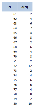
Another reason for using 72 over other close numbers is that 72 has a lot of divisors, in particular out of all the integers within 10 of 72, 72 has the most divisors. The following table displays the divisors function d(n), for values of n between 60 and 80. 72 clearly stands out as a good candidate.

​The rule of 72 in Actuarial Modelling

The main use I find for this trick is in mentally adjusting historic claims for claims inflation. I know that if I put in 6% claims inflation, my trended losses will double in size from their original level approximately every 12 years. Other uses include when analysing investment returns, thinking about the effects of monetary inflation, or it can even be useful when thinking about the effects of discounting.
​
Can we apply the Rule of 72 anywhere else?

As an aside, we should be careful when attempting to apply the rule of 72 over too long a time period. Say we are watching a movie set in 1940, can we use the Rule of 72 to estimate what values in the movie are equivalent to now? Let's set up an example and see why it doesn't really work in practice. Let's suppose an item in our movie costs 10 dollars.  First we need to pick an average inflation rate for the intervening period (something in the range of 3-4% is probably reasonable). We can then reason as follows; 1940 was 80 years ago, at 4% inflation, $\frac{72}{4} = 18$, and we’ve had approx. 4 lots of 18 years in that time. Therefore the price would have doubled 4 times, or will now be a factor of 16. Suggesting that 10 dollars in 1940 is now worth around 160 dollars in today's terms.

It turns out that this doesn’t really work though, let’s check it against another calculation. The average price of a new car in 1940 was around 800 dollars and the average price now is around 35k, which is a factor of 43.75, quite a bit higher than 16. The issue with using inflation figures like these over very long time periods, is for a given year the difference in the underlying goods is fairly small, therefore a simple percentage change in price is an appropriate measure. When we chain together a large number of annual changes, after a certain number of years, the underlying goods have almost completely changed from the first year to the last. For this reason, simply multiplying an inflation rate across decades completely ignores both improvements in the quality of goods over time, and changes in standards of living, so doesn't really convey the information that we are actually interested in.
​

​There is a way of thinking about probability distributions that I’ve always found interesting, and to be honest I don’t think I’ve ever seen anyone else write about it. For each  probability distribution, the CDF can be thought of as a partial infinite sum, or partial integral identity, and the probability distribution is uniquely defined by this characterisation (with a few reasonable conditions)

I think at this point most people will either have no idea what I'm talking about (probably because I've explained it badly), or they’ll think what I’ve just said is completely obvious. Let me give an example to help illustrate.

Poisson Distribution as a partial infinite sum

Start with the following identity:

And let's bring the exponential over to the other side.

$$ \sum_{i=0}^{\infty} \frac{ x^i}{i!} e^{-x}  = 1$$

Let's state a few obvious facts about this equation; firstly, this is an infinite sum (which I claimed above were related to probability distributions - so good so far). Secondly, the identity is true by the definition of $e^x$, all we need to do to prove the identity is show the convergence of the infinite sum, i.e. that $e^x$ is well defined. Finally, each individual summand is greater than or equal to 0.

With that established, if we define a function:

$$ F(x;k) = \sum_{i=0}^{k} \frac{ x^i}{i!} e^{-x}$$

That is, a function which specifies as its parameter the number of partial sumummads we should add together. We can see from the above identity that:

• The partial sum is strictly less than 1
• The sum converges to 1 as $k \rightarrow \infty$.

But wait, the formula for $F(x;k)$ above is actually just the formula for the CDF of a Poisson random variable! That’s interesting right? We started with an identity involving an infinite sum, we then normalised it so that the sum was equal to 1, then we defined a new function equal to the partial summation from this normalised series, and voila, we ended up with the CDF of a well-known probability distribution.

Can we repeat this again? (I’ll give you a hint, we can)

Exponential Distribution as a partial infinite integral

Let’s examine an integral this time. We’ll use the following identity:

$$\int_{0}^{ \infty}  e^{- \lambda x} dx = \lambda$$
 
An integral is basically just a type of infinite series, so let’s apply the same process, first we normalise:
 
$$ \frac{1}{\lambda}  \int_{0}^{ \infty}  e^{- \lambda x} dx = 1$$
 
Then define a function equal to the partial integral:

$$ F(y) = \frac{1}{\lambda}  \int_{0}^{ y}  e^{- \lambda x} dx $$

And we've ended up with the CDF of an Exponential distribution!

Euler Integral of the first kind

This construction even works when we use more complicated integrals. The Euler integral of the first kind is defined as:

This allows us to normalise:

$$\frac{\int_{0}^{1}t^{{x-1}}(1-t)^{{y-1}}dt}{B(x,y)} = 1$$

And once again, we can construct a probability distribution:

$$B(x;a,b) = \frac{\int_{0}^{x}t^{{a-1}}(1-t)^{{b-1}}dt}{B(a,b)}$$

Which is of course the definition of a Beta Distribution, this definition bears some similarity to the definition of an exponential distribution in that our normalisation constant is actually defined by the very integral which we are applying it to.

Conclusion

So can we do anything useful with this information? Well not particularly. but I found it quite insightful in terms of how these crazy formulas were discovered in the first place, and we could potentially use the above process to derive our own distributions – all we need is an interesting integral or infinite sum and by normalising and taking a partial sum/integral we've defined a new way of partitioning the unit interval.

Hopefully you found that interesting, let me know if you have any thoughts by leaving a comment in the comment box below!

​I saw a useful way of parameterising the Beta Distribution a few weeks ago that I thought I'd write about.

The standard way to define the Beta is using the following pdf:

​Where $ x \in [0,1]$ and $B( \alpha, \beta ) $ is the Beta Function:

​When we use this parameterisation, the first two moments are:

​We see that the mean and the variance of the Beta Distribution depend on both parameters - $\alpha$ and $\beta$. If we want to fit these parameters to a data set using a method of moments then we need to use the following formulas, which are quite complicated:

This is not the only possible parameterisation of the Beta Distribution however. ​We can use an alternative definition where we define:

And then by construction, $E[X] = \gamma$, and we can calculate the new variance:

Placing these new variables back in our pdf gives the following equation:

So why would we bother to do this? Our new formula now looks more complicated to work with than the one we started with. There are however two main advantages to this new version, firstly the method of moments is much simpler to set up, our first parameter is simply the mean, and the formula for variance is easier to calculate than before. This makes using the Beta distribution much easier in a Spreadsheet. The second advantage, and in my mind the more important point, is that since we now have a strong link between the central moments and the two parameters that define the distribution we now have an easy and intuitive understand of what our parameters actually represent.
​
As I’ve written about before, rather than just sticking with the standard statistics textbook version, I’m a big fan of pushing parameterisations that are both useful and easily interpretable, The version of the Beta Distribution presented above achieves this. Furthermore it also fits nicely with the schema I've written about before (most recently in the in the post below on negative binomial distribution), in which no matter which distribution we are talking about, the first parameter of a distribution gives you information about it's mean, the second parameter  gives information about its volatility, etc. By doing this you give yourself the ability to compare distributions and sense check parameterisations at a glance.

If you have ever generated Random Variables stochastically using a Gaussian Copula, you may have noticed that the correlation of the generated sample ends up being lower than the value of the Covariance matrix of the underlying multivariate Gaussian Distribution. For an explanation of why this happens you can check out a previous post of mine:
www.lewiswalsh.net/blog/correlations-friedrich-gauss-and-copula.

It would be nice if we could amend our method to compensate for this drop. As a quick fix, we can simply run the model a few times and fudge the Covariance input until we get the desired Correlation value. If the model runs quickly, this is quite easy to do, but as soon as the model starts to get bigger and slower, it quickly becomes impractical to run it three of four times just to get the output Correlation we desire.

We can do better than this. The insight we rely on is that for a Gaussian Copula, the Pearson Correlation in the generated sample just depends on the Covariance Value. We can therefore create a precomputed table of Input and Output values, and use this to select the correct input value for the desired output. I wrote some R code to do just that, we compute a table of Pearson's Correlations obtained for various Input Covariance values when using the Gaussian Copula.

a <- library(MASS)
library(psych)

set.seed(100)

m <- 2
n <- 10^6

OutputCor <- 0
InputCor <- 0

for (i in 1:100) {
  
  sigma <- matrix(c(1, i/100,
                    i/100, 1), 
                  nrow=2)
  z <- mvrnorm(n,mu=rep(0, m),Sigma=sigma,empirical=T)
  
  u <- pnorm(z)
  
  OutputCor[i] <- cor(u,method='pearson')[1,2]
  InputCor[i] <- i/10
  
}

OutputCor
InputCor

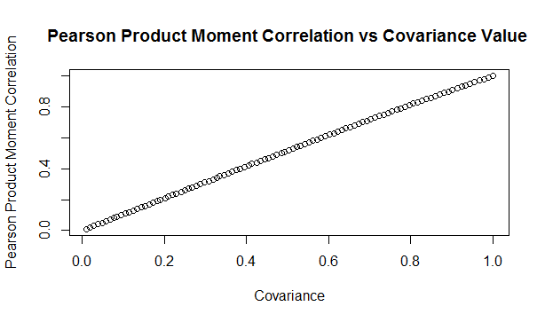
Here is a sample from the table of results. You can see that the drop is relatively modest, but it does apply consistent across the whole table.

Here is a graph showing the drop in values:
​

Updated Algorithm

We can then use the pre-computed table, interpolating where necessary, to give us a Covariance value for our Multivariate Gaussian Distribution which will generate the desired Pearson Product Moment Correlation Value. So for example, if we would like to generate a sample with a Pearson Product Moment value of $0.5$, according to our table, we would need to use $0.517602$ as an input Covariance. We can test these values using the following code:

a <- library(MASS)
library(psych)

set.seed(100)

m <- 2
n <- 5000000
sigma <- matrix(c(1, 0.517602,
                  0.517602, 1), 
                nrow=2)
z <- mvrnorm(n,mu=rep(0, m),Sigma=sigma,empirical=T)
u <- pnorm(z)

cor(u,method='pearson')

​Analytic Formulas

I tried to find an analytic formula for the Product Moment values obtained in this manner, but I couldn't find anything online, and I also wasn't able to derive one myself. If we could find one, then instead of using the precompued table, we would be able to simply calculate the correct value. While searching, I did come across a number of interesting analytic formulas linking the values of Kendall's Tau, Spearman's Rank, and the input Covariance..

All the formulas below are from Fang, Fang, Kotz (2002) Link to paper: 
www.sciencedirect.com/science/article/pii/S0047259X01920172

The paper gives the following two results, where $\rho$ is the Pearson's Product Moment

We can then use these formulas to extend our method above further to calculate an input Covariance to give any desired Kendall Tau, or Spearman's Rank. I initially thought that they would link the Pearson Product Moment value with Kendall or Spearman's measure, in which case we would still have to use the precomputed table. After testing it I realised that it is actually linking the Covariance to Kendall and Spearman's measures.

Thinking about it, Kendall's Tau, and Spearman's Rank are both invariant to the reverse Gaussian transformation when moving from $z$ to $u$ in the algorithm. Therefore the problem of deriving an analytic formula for them is much simpler as one only has to link their values for a multivariate Gaussian Distribution. Pearson's however does change, therefore it is a completely different problem and may not even have a closed form solution.

As an example of how to use the above formula, suppose we'd like our generated data to have a Kendall's Tau of $0.4$. First we need to invert the Kendall's Tau formula:

$$ \rho = sin ( \frac{ \tau \pi }{2} ) $$

We then plug in $\rho = 0.4 $ giving:

​We can then test this value with the following R code:

a <- library(MASS)
library(psych)

set.seed(100)

m <- 2
n <- 50000
sigma <- matrix(c(1, 0.587785,
                  0.587785, 1), 
                nrow=2)
z <- mvrnorm(n,mu=rep(0, m),Sigma=sigma,empirical=T)
u <- pnorm(z)
cor(z,method='kendall')

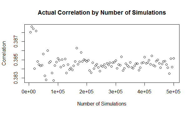
Which we see gives us the value of $\tau$ we want. In this case the difference between the input Covariance $0.587785$, and the value of Kendall's Tau $0.4$ is actually quite significant.

It's the second week of your new job Capital Modelling job. After days spent sorting IT issues, getting lost coming back from the toilets, and perfecting your new commute to work (probability of getting a seat + probability of delay * average journey temperature.) your boss has finally given you your first real project to work on.

You've been asked to carry out an annual update of the Underwriting Risk Capital Charge for a minor part of the company's Motor book. Not the grandest of analysis you'll admit, this particular class only makes up about 0.2% of the company's Gross Written Premium, and the Actuaries who reserve the company's bigger classes would probably consider the number of decimal places used in the annual report more material than your entire analysis. But you know in your heart of hearts that this is just another stepping stone on your inevitable meteoric rise to Chief Actuary in the Merger and Acquisition department, where one day you will pass judgement on billion dollar deals in-between expensive lunches with CFOs, and drinks with journalists on glamorous rooftop bars.

The company uses in-house reserving software, but since you're not that familiar with it, and because you want to make a good impression, you decide to carry out extensive checking of the results in Excel. You fire up the Capital Modelling Software (which may or may not have a name that means a house made out of ice), put in your headphones and grind it out.

Hours later you emerge triumphant, and you've really nailed it, your choice of correlation (0.4), and correlation method (Gaussian Copula) is perfect. As planned you run extracts of all the outputs, and go about checking them in Excel. But what's this? You set the correlation to be 0.4 in the software, but when you check the correlation yourself in Excel, it's only coming out at 0.384?! What's going on?

Simulating using Copulas

The above is basically what happened to me (minus most of the actual details. but I did set up some modelling with correlated random variables and then checked it myself in Excel and was surprised to find that the actual correlation in the generated output was always lower than the input.) I looked online but couldn't find anything explaining this phenomenon, so I did some investigating myself.

So just to restate the problem, when using Monte Carlo simulation, and generating correlated random variables using the Copula method. When we actually check the correlation of the generated sample, it always has a lower correlation than the correlation we specified when setting up the modelling.

My first thought for why this was happening was that were we not running enough simulations and that the correlations would eventually converge if we just jacked up the number of simulations. This is the kind of behaviour you see when using Monte Carlo simulation and not getting the mean or standard deviation expected from the sample. If you just churn through more simulations, your output will eventually converge. When creating Copulas using the Gaussian Method, this is not the case though, and we can test this.

I generated the graph below in R to show the actual correlation we get when generating correlated random variables using the Copula method for a range of different numbers of simulations. There does seem to be some sort of loose limiting behaviour, as the number of simulations increases, but the limit appears to be around 0.384 rather than 0.4.

The actual explanation

First, we need to briefly review the algorithm for generating random variables with a given correlation using the normal copula.

Step 1 - Simulate from a multivariate normal distribution with the given covariance matrix.

Step 2 - Apply an inverse gaussian transformation to generate random variables with marginal uniform distribution, but which still maintain a dependency structure

Step 3 - Apply the marginal distributions we want to the random variables generated in step 2

We can work through these three steps ourselves, and check at each step what the correlation is.

The first step is to generate a sample from the multivariate normal. I'll use a correlation of 0.4 though out this example. Here is the R code to generate the sample:

a <- library(MASS)
library(psych)

set.seed(100)

m <- 2
n <- 1000
sigma <- matrix(c(1, 0.4,
                  0.4, 1), 
                nrow=2)
z <- mvrnorm(n,mu=rep(0, m),Sigma=sigma,empirical=T)

​

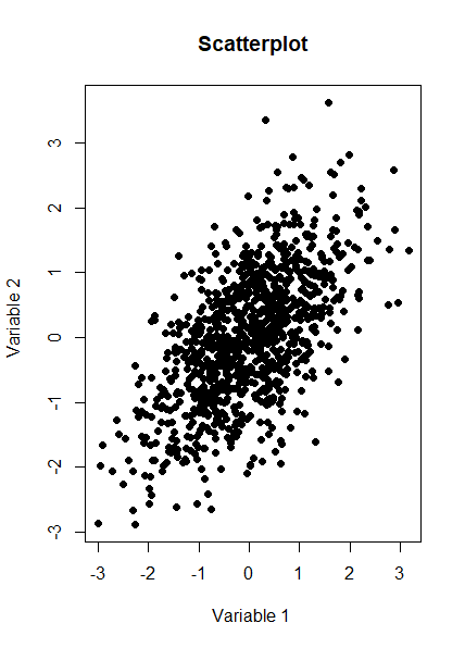
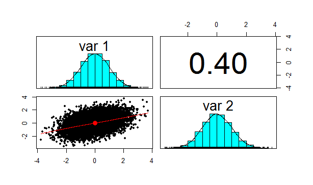
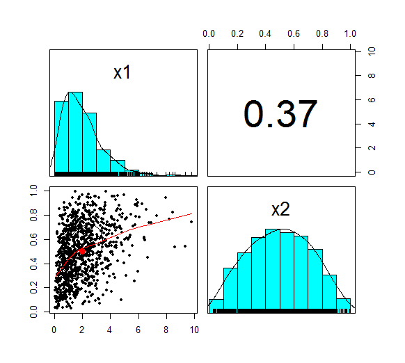
And here is a Scatterplot of the generated sample from the multivariate normal distribution:
​

We now want to check the product moment correlation of our sample, which we can do using the following code:
​

cor(z,method='pearson')

Which gives us the following result:

> cor(z,method='pearson')
     [,1] [,2]
[1,]  1.0  0.4
[2,]  0.4  1.0

So we see that the correlation is 0.4 as expected. The Psych package has a useful function which produces a summary showing a Scatterplot, the two marginal distribution, and the correlation:

Let us also check Kendall's Tau and Spearman's rank at this point. This will be instructive later on. We can do this using the following code:

cor(z,method='spearman')

cor(z,method='Kendall')

Which gives us the following results:

> cor(z,method='spearman')
          [,1]      [,2]
[1,] 1.0000000 0.3787886
[2,] 0.3787886 1.0000000

> cor(z,method='kendall')
          [,1]      [,2]
[1,] 1.0000000 0.2588952
[2,] 0.2588952 1.0000000

Note that this is less than 0.4 as well, but we will discuss this further later on.

We now need to apply step 2 of the algorithm, which is applying the inverse Gaussian transformation to our multivariate normal distribution. We can do this using the following code:

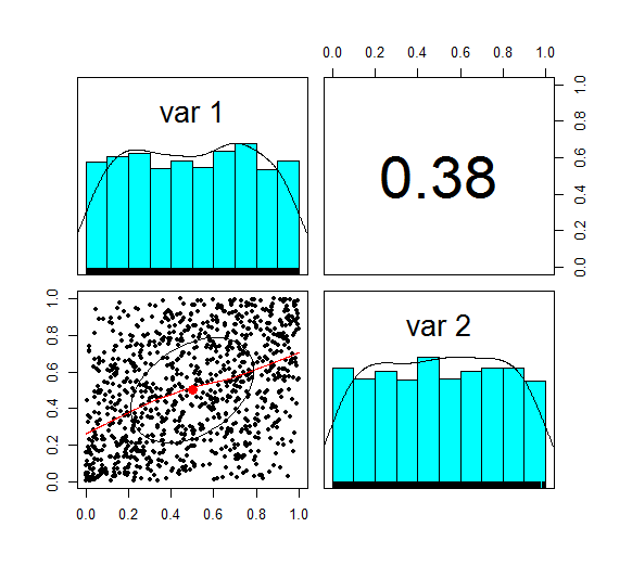
u <- pnorm(z)

We now want to check the correlation again, which we can do using the following code:

cor(z,method='spearman')

Which gives the following result:

> cor(z,method='spearman')
          [,1]      [,2]
[1,] 1.0000000 0.3787886
[2,] 0.3787886 1.0000000

​Here is the Psych summary again:

u is now marginally uniform (hence the name). We can see this by looking at the Scatterplot and marginal pdfs above.

We also see that the correlation has dropped to 0.379, down from 0.4 at step 1. The Pearson correlation measures the linear correlation between two random variables. We generated normal random variables, which had the required correlation, but then we applied a non-linear (inverse Gaussian) transformation. This non-linear step is the source of the dropped correlation in our algorithm.

We can also retest Kendall's Tau, and Spearman's at this point using the following code:

cor(z,method='spearman')

cor(z,method='Kendall')

This gives us the following result:

> cor(u,method='spearman')
          [,1]      [,2]
[1,] 1.0000000 0.3781471
[2,] 0.3781471 1.0000000

> cor(u,method='kendall')
          [,1]      [,2]
[1,] 1.0000000 0.2587187
[2,] 0.2587187 1.0000000

Interestingly, these values have not changed from above! i.e. we have preserved these measures of correlation between step 1 and step 2. It's only the Pearson correlation measure (which is a measure of linear correlation) which has not been preserved.

Let's now apply the step 3, and once again retest our three correlations. The code to carry out step 3 is below:

x1 <- qgamma(u[,1],shape=2,scale=1)
x2 <- qbeta(u[,2],2,2)

df <- cbind(x1,x2)
pairs.panels(df)

The summary for step 3 looks like the following.

This is the end goal of our method. We see that our two marginal distributions have the required distribution, and we have a correlation between them of 0.37. Let's recheck our three measures of correlation.
​

cor(df,method='pearson')

cor(df,meth='spearman')

cor(df,method='kendall')

> cor(df,method='pearson')
          x1        x2
x1 1.0000000 0.3666192
x2 0.3666192 1.0000000

> cor(df,meth='spearman')
          x1        x2
x1 1.0000000 0.3781471
x2 0.3781471 1.0000000

> cor(df,method='kendall')
          x1        x2
x1 1.0000000 0.2587187
x2 0.2587187 1.0000000

So the Pearson has reduced again at this step, but the Spearman and Kendall's Tau are once again the same.

Does this matter?

This does matter, let's suppose you are carrying out capital modelling and using this method to correlate your risk sources. Then you would be underestimating the correlation between random variables, and therefore potentially underestimating the risk you are modelling.

Is this just because we are using a Gaussian Copula? No, this is the case for all Copulas. Is there anything you can do about it? Yes, one solution is to just increase the input correlation by a small amount, until we get the output we want.

A more elegant solution would be to build this scaling into the method. The amount of correlation lost at the second step is dependent just on the input value selected, so we could pre-compute a table of input and output correlations, and then based on the desired output, we would be able to look up the exact input value to use.   

I was thinking about this last week at work when I was coding part of a model involving the parameters of a truncated lognormal distribution. The lognormal distribution definitely feels like it was named the wrong way round.
​
What is a Log-normal Distribution?

In other words, a Log-normal distribution is a distribution such that the log of the distribution is a normal distribution. It is not, as you might think, a distribution which is the log of the normal distribution.

So if $Y \sim N( \mu , {\sigma}^2 ) $ then $Log ( Y ) $ is not a lognormal distribution, instead $ e ^ Y $ is a lognormal distribution.

So to create a lognormal distribution, we don't take the log of the normal distribution, we take the exponential!
​
Why does this matter?

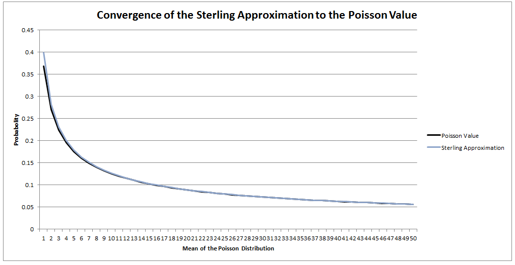
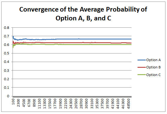
"The safest way to double you money is to fold it in half" Kin Hubbard

"I like to play Blackjack. I'm not addicted to gambling. I'm addicted to sitting in a semi-circle." Mitch Hedberg

Gambling is a risky business, in the long run everyone loses. Well not everyone. Bookmakers always seem to do alright. How is it that bookmakers make so much money out of gambling then? Is it through their superior wit and street smarts, or is there something else going on? It turns out that the method used by bookmakers involves a lot less insight and risk than you might think. The process is mathematical, and is guaranteed to turn a profit, and actually quite interesting.

Making a Dutch Book

Let's start with an example, suppose I am a bookmaker offering odds on the Super Bowl coin toss. We all know that for a fair coin, the probability of getting a heads is 50%, and the probability of getting tails is 50%.

We might suppose therefore that we would set our odds at 1/1, meaning for a bet of £1 if you win, you get £1 back plus your original £1. This means that you would double your money if you win (which happens about half the time) and lose all your money if you lose (which happens about half the time). Over time, if you made lots of bets of £1 at these odds, you would expect to break even.

Let's suppose though, that for reasons unknown to us, far more money is being bet on heads than tails. For example, suppose £1,000 is put on heads, and only £500 is put on tails. We can then examine our position under two scenarios, one where heads wins, and one where tails wins.

We have taken in £1,500 in total, and our outgoings are either £2,000 or £1,000. Making us a profit of £500 half the time, and -£500 half the time. Given each outcome is equally likely, over the long run if we keep offering odds like these we will expect to break even.

We can do better than this though. We can actually set the odds so that we break even every single time, not just in the long run. In order to see this, let's suppose that we change the odds so that they are 1/2 for heads, and 2/1 for tails. So that means, for every £2 bet on heads, we will pay out £1, plus the original £2 bet, and for every £1 bet on tails, we will pay out £2, plus the original £1 bet. Under these new odds, we would then end up with the following position:

We see now that because of how we have amended the odds, we don't actually care who wins. We will always pay out the same amount. The Bookmaker can then adjust the odds slightly, so that they will always pays out less than they have taken in. For example, they might offer 5/11 for heads, and 9/5 for tails. Under these odds, not only will the Bookmaker not care who wins, but they will always make a small margin on all bets placed. The exact figures in this case would be:

So we see that the Bookmaker has a foolproof system of always making money from gambling, and plus, they don't even need to be good at predicting who will win.

Irrational odds?

Isn't it crazy to offer odds of 2/1 on a coin toss though? We all know​ that the actual odds for a fair coin should be 1/1! The answer is that as soon as people see these odds, they should start betting on tails, and by supply and demand the odds for tails will start to move down, and the odds for heads will start to move up.

The bookmaker themselves might also decide to take a position at these odds and effectively bet money themselves by allowing the payout to be skewed towards a 50/50 split, giving their payout a positive Expected Value.

The first time I read about this system of bookmaking was in the book "Financial Calculus: an introduction to derivative pricing" by Baxter and Rennie, which I was reading in preparation for the IFoA ST6 exam. Baxter and Rennie brought it up because Bookmakers are actually undertaking a form of arbitrage, similar to the series of  notional trades used when deriving the price of futures contracts. You can see the similarities by simply noting that both the bookmaker and the derivatives trader are acting so as to not have any exposure to the actual value of the underlying event. By doing this, they don't actually need to take a view at all on what the expected outcome is, but they can instead exploit the relative values of different parts of the market.

What margin to online bookmakers charge?

I had a quick look at some odds offered by online bookmakers on a couple of events. One of the events I looked at was UFC 218. BestFightOdds.com gives a comparison of the odds offered by various betting websites. This is mainly to help people pick which website to bet on in order to get the best odds, but we can use it to compare the margins that the different websites charge. Assuming an equal bet is placed on each fight on the card, I calculated the following margins for the websites listed by BestFightOdds:

They range from a low of 2.62%, up to about 6%. The individual margin on each fight varies quite a bit, and also I suspect each website will run different margins on different sports and different events. The reason for this is that some of the higher margin websites might offer more incentives, and more free bets than the lower margin websites., plus they might be more established and spend more on advertising allowing them to charge more and still retain sufficient numbers of customers.

The fact that websites run margins does mean that if you are going to make money gambling you need to first beat the margin before you can even break even. Let's say you're really good at gambling and you can out-predict the market by 2%, you would still lose money overall gambling on any of these websites, because you also need to factor in the margin (also called the vig) that the websites charge.

Sources:

(1) BestfightOdds.com:
www.bestfightodds.com/events/ufc-218-holloway-vs-aldo-2-1368

​I saw a cool trick the other day involving the Poisson Distribution and Stirling's Approximation.

Given a Poisson Distribution $ N  $ ~ $ Poi( \lambda ) $

The probability that $N$ is equal to a given $n$ is defined to be:

$$P ( N = n) = \frac { {\lambda}^n e^{-n} } {n! } $$
What is the probability that $N$ is equal to it's mean? In this case, let's use $n$ as the mean of the distribution for reasons that will become clear later.

Plugging $n$ into the definition of the Poisson distribution gives:

$$P ( N = n) = \frac { n^n e^{-n} } {n! } $$
At this point, we use Sterling's approximation. Which states that for large $n$:

                                                             $n!$  ~ $ {\left( \frac { n } {e } \right) }^n \frac { 1 } { \sqrt{ 2 \pi n } }$

Plugging this into the definition of the Poission Distribution gives:

$$P ( N = n) = \frac { n^n e^{-n} } {{\left( \frac { n } {e } \right) }^n} \frac { 1 } { \sqrt{ 2 \pi n } } $$
Which simplifies to:

$$P ( N = n) = \frac { 1 } { \sqrt{ 2 \pi n } } $$

So for large $n$ we end up with a nice result for the Probability that a Poisson Distribution will end up being equal to it's Expected Value.

Convergence

The convergence of the series is actually really quick. I checked the convergence for n between 1 and 50, and even by n=5, the approximation is very close, when I graphed it, the lines become indistinguishable very quickly.
​

I always found it quite interesting that prior to the 19th century, Probability Theory was basically just a footnote to the study of gambling. The first time that Probability Theory was formalised in any systematic way at all was through the correspondence of three 17th century mathematicians, Pierre Fermat (famous for his last theorem), Blaise Pascal (famous for his wager), and Gerolamo Cardano (not actually famous at all) when analysing a problem in gambling called the problem of points. 

The problem of points is the problem of how to come up with a fair way to divide the winnings when betting on a game of chance which has interrupted before it can be finished. For example, let's say we are playing a game where we take it in turns to roll a dice and we record how many 6s we get, the first person who rolls a total of 10 6s wins. What happens if we are unable to finish the game, but one player has already rolled 8 6s, whereas their opponent has only rolled 2 6s. How should we divide the money in a fair way? Obviously it's unfair to just split the money 50-50 as the player with 8 6s has a much higher chance of winning, but at the same time, there is a chance that the player with only 2 6s might get lucky and still win, so we can't just give all the money to the player who is currently winning. The solution to the problem involves calculating the probability of each player winning given their current state, and then dividing the money proportionally. In order to answer this question in a systematic way, Fermat, Pascal, and Cardano formalised many of the basic principles of Probability Theory which we still use today.

Newton - Pepys Problem

The Newton - Pepys problem is another famous problem related to gambling and Probability Theory. It is named after a series of correspondence between Isaac Newton and Samuel Pepys, the famous diarist, in 1693. Pepys wrote to Newton asking for his opinion on a wager that he wanted to make.

Which of the following three propositions has the greatest chance of success?
A. Six fair dice are tossed independently and at least one “6” appears.
B. Twelve fair dice are tossed independently and at least two “6”s appear.
C. Eighteen fair dice are tossed independently and at least three “6”s appear.

Pepys initially believed that Option C had the highest chance of success, followed by Option B, then Option A. Newton correctly answered that it was in fact the opposite order and that Option A was the most likely, Option C was the least likely.

Wikipedia has the analytical solution to the problem. Which comes out as:

We can clearly see from this graph that Option A is the most likely Option of the three, with Option C being the least likely. We can tell all of this by just setting up a model that takes 5 minutes to build and give an answer in seconds. It makes you wonder what Newton would have been able to manage if he had access to the computing power that we take for granted now.

Sources:
Wikipedia: en.wikipedia.org/wiki/Newton%E2%80%93Pepys_problem
An Article by Stephen Stigler: arxiv.org/pdf/math/0701089.pdf

I could be on my own here, but personally I always thought the definition of Sample Standard Deviation is pretty ugly.
$$ \sqrt {\frac{1}{n - 1} \sum_{i=1}^{n} { ( x_i - \bar{x} )}^2 } $$
We've got a square root involved which can be problematic, and what's up with the $\frac{1}{n-1}$? Especially the fact that it's inside the square root, also why do we even need a separate definition for a sample standard deviation rather than a population standard deviation?

When I looked into why we do this, it turns out that the concept of sample standard deviation is actually a bit of a mess. 

Before we tear it apart too much though, let's start by looking at some of the properties of  standard deviation which are good.

Advantages of Standard Deviation
​

• Unlike the variance, the standard deviation is in the same units as the mean. For example, if we are measuring the height of people in meters, if we take the mean, then the units will also be in meters (which probably sounds so obvious you wouldn't even think about it), the variance of heights on the other hand will be in meters squared which can be problematic. This is why we use the standard deviation which will convert the units back to meters.
• We can fully characterise many distributions by just specifying the mean and standard deviation. This is the case for many major distributions for example the Normal Distribution, Log-normal, Exponential, etc.
• In order to compare the variability of two distributions, we need a dimensionless quantity representing variability which is not effected by the absolute size of the underlying data. For example, if we are trying to answer the question: 'which has more variability, human height, or dog height', then if we just look at the variance of both of these, since humans are much taller in general the variance will also be greater and we might mistakenly believe that there is more variability in human height. If instead we look at the Coefficient of Variation, which is defined to be Standard Deviation over Mean, then this will be unaffected by the greater average human height and we would find out that there is actually greater relative variability in dog size (I would guess this is the case, but I've not actually checked it).
• The Sample Standard Deviation is an unbiased estimator of the population standard Deviation.

​
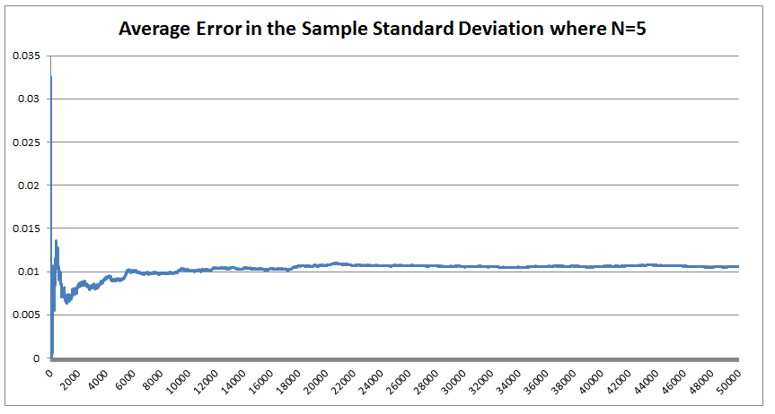
The last property is a really important one. The $\frac{1}{n-1}$ factor is a correction we make which we are told turns the sample standard deviation into an unbiased estimator of the population standard deviation. We can test this pretty easily, I sampled 50,000 simulations from a probability distribution and then measured the squared difference between the mean of the sample standard deviation and the actual value computed analytically.​​

We see that the Average Error converges quite quickly but for some reason it doesn't converge to 0 as expected!

It turns out that the usual formula for the sample standard deviation is not actually an unbiased estimator of the population standard deviation after all. I'm pretty sure they never mentioned that in my stats lectures at uni. The $n-1$ correction changes the formula for sample variance into an unbiased estimator, and the formula we use for the sample standard deviation is just the square root of the unbiased estimator for variance. If we do want an unbiased estimator for the sample standard deviation then we need to make an adjustment based not just on the sample size, but also the underlying distribution. Which in many cases we are not going to know at all.

The wiki page has a good summary of the problem, and also has formulas for the unbiased estimator of the sample standard deviation:
en.wikipedia.org/wiki/Unbiased_estimation_of_standard_deviation
​
Just to give you a sense of the complexity, here is the factor that we need to apply to the usual definition of sample standard deviation in order to have an unbiased estimator for a normal distribution.
$$ \frac {1} {    \sqrt{  \frac{2}{n-1}   }  \frac{  \Gamma \Big( \frac{ n } {2} \Big) }  {\Gamma \Big(  \frac{n-1}{2} \Big)}   }  $$

Where $\Gamma$ is the Gamma function.

​Alternatives to Standard Deviation

Are there any obvious alternatives to using standard deviation as our default measure of variability? Nassim Nicholas Taleb, author of Black Swan, is also not a fan of the wide spread use of the standard deviation of a distribution as a measure of its volatility. Taleb has different issues with it, mainly around the fact that it was often overused in banking by analysts who thought it completely characterised volatility. So for example, when modelling investment returns, an analyst would look at the sample standard deviation, and then assume the investment returns follow a Lognormal distribution with this standard deviation, when we should actually be modelling returns with a much fatter tailed distributions. So his issue was the fact that people believed that they were fully characterising volatility in this way, when they should have also been considering kurtosis and higher moments or considering fatter tailed distributions. Here is a link to Taleb's rant which is entertaining as always:

www.edge.org/response-detail/25401

Taleb's suggestion is a different statistic called Mean Absolute Deviation the definition is.
$$\frac{1}{n} \sum_{i=1}^n | x_i - \bar{x} | $$

We can see immediately why mathematicians prefer to deal with the standard deviation instead of the mean absolute deviation, working with sums of absolute values is normally much more difficult analytically than working with the square root of the sum of squares. In the ages of ubiquitous computing though, this should probably be a smaller consideration.

Designing a new number system

I got interested in alternative number systems when I read Malcolm Gladwell's book Outliers back in uni. You might be surprised that Gladwell would write about this topic, but he actually uses it to attempt to explain why Asian students tend to do so well at maths in the US. I was flicking through an old notebook the other day and I can across my attempt at designing such a system. I thought it might be interesting to write up my system. 

To set the scene, here is the relevant extract from the book:

"Take a look at the following list of numbers: 4,8,5,3,9,7,6. Read them out loud to yourself. Now look away, and spend twenty seconds memorizing that sequence before saying them out loud again.If you speak English, you have about a 50 percent chance of remembering that sequence perfectly If you’re Chinese, though, you’re almost certain to get it right every time. Why is that? Because as human beings we store digits in a memory loop that runs for about two seconds. We most easily memorize whatever we can say or read within that two second span. And Chinese speakers get that list of numbers—4,8,5,3,9,7,6—right every time because—unlike English speakers—their language allows them to fit all those seven numbers into two seconds.

That example comes from Stanislas Dehaene’s book “The Number Sense,” and as Dehaene explains:
Chinese number words are remarkably brief. Most of them can be uttered in less than one-quarter of a second (for instance, 4 is ‘si’ and 7 ‘qi’) Their English equivalents—”four,” “seven”—are longer: pronouncing them takes about one-third of a second. The memory gap between English and Chinese apparently is entirely due to this difference in length. In languages as diverse as Welsh, Arabic, Chinese, English and Hebrew, there is a reproducible correlation between the time required to pronounce numbers in a given language and the memory span of its speakers. In this domain, the prize for efficacy goes to the Cantonese dialect of Chinese, whose brevity grants residents of Hong Kong a rocketing memory span of about 10 digits.

It turns out that there is also a big difference in how number-naming systems in Western and Asian languages are constructed. In English, we say fourteen, sixteen, seventeen, eighteen and nineteen, so one would think that we would also say one-teen, two-teen, and three-teen. But we don’t. We make up a different form: eleven, twelve, thirteen, and fifteen. Similarly, we have forty, and sixty, which sound like what they are. But we also say fifty and thirty and twenty, which sort of sound what they are but not really. And, for that matter, for numbers above twenty, we put the “decade” first and the unit number second: twenty-one, twenty-two. For the teens, though, we do it the other way around. We put the decade second and the unit number first: fourteen, seventeen, eighteen. The number system in English is highly irregular. Not so in China, Japan and Korea. They have a logical counting system. Eleven is ten one. Twelve is ten two. Twenty-four is two ten four, and so on.
That difference means that Asian children learn to count much faster. Four year old Chinese children can count, on average, up to forty. American children, at that age, can only count to fifteen, and don’t reach forty until they’re five: by the age of five, in other words, American children are already a year behind their Asian counterparts in the most fundamental of math skills.

The regularity of their number systems also means that Asian children can perform basic functions—like addition—far more easily. Ask an English seven-year-old to add thirty-seven plus twenty two, in her head, and she has to convert the words to numbers (37 + 22). Only then can she do the math: 2 plus 7 is nine and 30 and 20 is 50, which makes 59. Ask an Asian child to add three-tens-seven and two tens-two, and then the necessary equation is right there, embedded in the sentence. No number translation is necessary: It’s five-tens nine.

“The Asian system is transparent,” says Karen Fuson, a Northwestern University psychologist, who has done much of the research on Asian-Western differences. “I think that it makes the whole attitude toward math different. Instead of being a rote learning thing, there’s a pattern I can figure out. There is an expectation that I can do this. There is an expectation that it’s sensible. For fractions, we say three fifths. The Chinese is literally, ‘out of five parts, take three.’ That’s telling you conceptually what a fraction is. It’s differentiating the denominator and the numerator.”

The much-storied disenchantment with mathematics among western children starts in the third and fourth grade, and Fuson argues that perhaps a part of that disenchantment is due to the fact that math doesn’t seem to make sense; its linguistic structure is clumsy; its basic rules seem arbitrary and complicated.

Asian children, by contrast, don’t face nearly that same sense of bafflement. They can hold more numbers in their head, and do calculations faster, and the way fractions are expressed in their language corresponds exactly to the way a fraction actually is—and maybe that makes them a little more likely to enjoy math, and maybe because they enjoy math a little more they try a little harder and take more math classes and are more willing to do their homework, and on and on, in a kind of virtuous circle.

When it comes to math, in other words, Asians have built-in advantage. . ."

Here's a link to Gladwell's website which contains the extract.
gladwell.com/outliers/rice-paddies-and-math-tests/

Base-10 System

Gladwell mainly talks about the words that the Chinese use for numbers and the structure inherent in them, but there is actually another more interesting way we can embed structure in our number system.

Our current number system is base-10, which means that we have different symbols for all the numbers up to 10 (0,1,2,3,4,...,9), and then when we get to the number 10, we use the first number again but we move it over one place, and then put a zero in it's place. When we are teaching a child how to write numbers, this is exactly how we explain it to them. For example to write two hundred and seven, we would tell them that they need to put a 2 in the hundreds columns a 0 in the tens column and a 7 in the units column - 207.

The fact that we use a base-10 number system is actually just a historical quirk. The only reason humans started to use it is just that we have 10 fingers, there's no particular mathematical benefit to a base-10 system. We could actually base our number system on any integer. The most commonly used alternative is the binary number system used extensively in computing. The binary number system is a base-2 number system where we only have 2 symbols - 0 and 1. The trick is that instead of reusing the first symbol when we get to ten, we do it when we get to two. So the sequence of numbers up to 10 in binary is:

In fact we don't even need to restrict ourselves to integers as the base of our number system. For example, we could even use base $ \pi $! Under this system if we want to write $ \pi $, then we would just write 1, to write $ \pi^2 $ it would just be 10. Writing one in base $ \pi $ would be quite difficult though, and we would need to either write $ 1 / {\pi} $ or invent a new character.



Base 12 number system

So what would be the ideal number on which to base our number system?

I'm going to make the argument that a base 12 number system would be the best option. 12 has a large number of small factors and this makes it ideal as a base.

• 12 has almost twice as many prime factors as 10. When working in base 10, it is relatively easy to multiply a number by either 2, 5, or 10, this is because these are all factors of 10. When we are working in base 12, it will be easy to multiply by 2, 3, 4, 6, and 12. Division by these numbers is also much easier. 
• It is the smallest number divisible by 1,2,3, and 4.
• We seem to intuitively favour the number 12 in many common circumstances. It has it's own name - a dozen, we also used it to split inches into feet. It's actually the largest integer that has still has it's own name. Once we get to 13, it's just a combination of three and teen, and so on for larger numbers, but eleven and twelve have their own names.
• We have 12 knuckles on the four fingers of each hand (ignoring thumbs) making counting on our hands easy still.

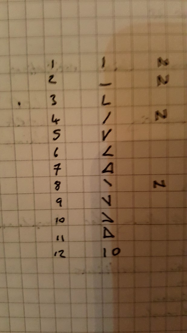
Returning back to Gladwell's idea, another change we could make to the number system to help make it more structured is to change the actual symbols we use for the integers. Here was my attempt from 2011 for alternative symbols we could use.

My approach was to embed as much structure into the numbers as possible, so the symbol for three is actually just a combination of the symbols for one and two. This applies for all the numbers other than one, two, four, and eight.

I wonder if it would be possible to come up with some sort of rule about how the symbols rotate to further reduce the total number of symbols and also to add some additional structure to the symbols.

Let me know if you can think of any additional improvements that could be made to our number system.
​

I think the first time I read about the Difference Engine was actually in the novel of the same name by William Gibson and Bruce Sterling. The book is an alternative history, set in the 19th centuary where Charles Babbage, actually finished building the Difference Engine, a Mechanical calculator he designed. This in turn lead to him getting funding for the Analytical Engine, a Turing-complete mechanical computer which Babbage also designed in real life, but also didn't actually finish building. I really enjoyed the book, but how plausible was this chain of events? How did the Difference Engine work? And what problem was Babbage trying to solve when he came up with the idea for the Difference Engine?

Computers before Computers

Before electronic computers were invented, scientist and engineers were forced to use various tricks and short cuts to enable them to carry out difficult calculations by hand.  One short cut that was used extensively, and one which Babbage would have been very familiar with, was the use of log tables to speed up multiplication. A log tables is simply a table which lists the values of the logarithmic function. If like me you've never used a log table, then how are they useful?

Log Tables

The property of logarithms that makes them useful in simplifying certain calculations is that:

$ log(AB) = log(A) + log(B) $

We use this property often in number theory when we wish to turn a multiplicative problem in to an arithmetic problem and vice versa. In this case it's more straightforward though. If we want to calculate $A*B$ we can convert the figures into logs, and then we just need to add the logs together and convert back to obtain the value of $A*B$.

Lets say we want to calculate $ 134.7 * 253.9 $ . What we can do instead is calculate:

$ log( 134.7) = 2.1294 $ and $ log (253.9) = 2.4047 $

then we just need to add together​

and convert back from logs

​​​$ 10^{4.5340} = 34200 $

which we can easily verify as the number we require. 

Haven't we just made our problem even harder though? Before we needed to multiply two numbers, and now instead we need to do two conversions and an addition, admittedly it's easier to add two large numbers together than multiply them, but what about the conversion? The way around this is to have a book of the values of the log function so that we can just look up the log of any number we are interested in, allowing us to easily convert to and from logs.

This is probably a good point to introduce Charles Babbage properly, Babbage was an English Mathematician, Inventor, and Philosopher born in 1791. He was a rather strange guy, as well as making important contributions to Computer Science, Mathematics and Economics, Babbage founded multiple societies. One society was founded to investigate paranormal activity, one was founded to promote the use of Leibniz notation in calculus, and another was founded in an attempt to foster support for the banning of organ grinders.
​
When he wasn't keeping himself busy investigating the supernatural, Babbage was also a keen astronomer. Since astronomy is computation heavy, this meant that Babbage was forced to make extensive use of the log tables that were available at the time. These tables had all been calculated by hand by people called computers. Being a computer was a legitimate job at one point, they would sit and carry out calculations by hand all day every day, not the most exciting job if you ask me. Because the log tables had all been created by teams of human calculators, errors had naturally crept in. The tables were also very expensive to produce. This lead Babbage to conceive of a mechanical machine for calculating log tables, he called this invention the Difference Engine.

Method of differences

A difference engine uses the method of finite differences to calculate the integer values of polynomial functions. I remember noticing something similar to the method of finite differences when I was playing around trying to guess the formulas for sequences of integers at school. 

If someone gives you an integer sequence and they ask you to find the formula, say we are given,

$1,4,7,10,13,...$

Then, in this case, the answer is easy, we can see that we are just adding 3 each time. To make this completely obvious, we can write in the differences between the numbers..

1 - 4 - 7 - 10 - 13 - ...
  3    3    3    3

What if we are given a slightly more complex sequence though? For example:

$1,3,6,10,15,...$

This one is a bit more complicated, let's see what happens when we add in the differences again:

1 - 3 - 6 - 10 - 15
  2    3    4     5

Now we see that there is an obvious pattern in the number we are adding on each time. Looking at the differences between these numbers we see:

1 - 3 - 6 - 10 - 15
  2    3    4     5
      1    1    1

So what's happened here? We now have stability on the second level of the differences. It turns out that this is equivalent to the underlying formula being a quadratic. In this case the formula is $0.5*x^2+1.5x+1$. If we assume the first number in the sequence is equivalent to $x=0$ we can now easily recreate the sequence, and easily calculate the next value.

Let's try a difficult example, if we are given the following sequence and told to guess the next value, we can use a similar method to get the answer.

$2,5,18,47,98,177$

Setting up the method:

2 - 5 - 18 - 47 - 98 - 177
   3   13   29    51    79
     10  16    22    28
         6    6     6

Since we get a constant at the third level, this sequence must be a cubic, once we know this, it's much easier to guess what the actual formula is. In this case it is x^3-x^2-x+3. Babbage's insight was that we can calculate the next value in this sequence just by adding on another diagonal to this table of differences.

Adding $6$ to $28$ gives $34$, then adding $34$ to $79$ gives $113$, and then adding $113$ to $177$ gives us $290$. Which means that the next value in the sequence is $290$ So we get:

2 - 5 - 18 - 47 - 98 - 177 -  290
   3   13   29    51    79    113
     10  16   22    28    34
         6    6    6       6

As you might guess, this process generalises to higher order polynomials. For a given sequence, if we keep trying the differences of the differences and eventually get to a constant then we will know the sequence is formed by a polynomial, and we will also know the degree of the polynomial. So if you are ever a given an integer sequence and asked to find the pattern, always check the differences and see if it eventually becomes a constant, if it does, then you will know the order of the polynomial which defines the sequence and you will also be able to easily compute the next value directly.

So how does this apply to Babbage's difference engine?

The insight is that we have here a method of enumerating the integer values of a polynomial just using addition. Also at each stage we only need to store the values of the leading diagonal. And each polynomial is uniquely determined by specifying its differences.

The underlying message is that multiplication is difficult. In order to come up with a shortcut for multiplication, we use log tables to make the problem additive. And even further, we now have a method for calculating the log function which also avoids multiplication.

So given we have this method of calculating the integer values of a polynomial, how can we use this to calculate values of the log function?

​Approximating Functions

The obvious way to approximate a log function with a polynomial would be to just take its Taylor expansion.

For example, the Taylor expansion of $ log ( 1 - x ) $ is:

$ log ( 1 - x ) =  - \sum^{\infty}_{n=1} \frac{x^n}n $

There is a downside to using the Taylor expansion though. Given the mechanical constraints at the time, Babbagge's Difference Engine could only simulate a 7th degree polynomial. So how close can we get with a Taylor expansion? We can use Taylor's theorem to calculate the convergence of the approximation, but this will be quite a bit of work, and since we can easily calculate the actual value of the log function it's easier to just test the approximation with a computer. So taking $log(0.5)$ as an example, when I use a calculator, I am told that it equals $-0.6931$, but when I check the 7th order polynomial I get $-0.6923$, and it's not until I get to the 10th polynomial that we are accurate even to 4 digits.
​
If we require a more accurate approximation, we will have to use numerical methods in conjunction with a restriction on the range of convergence. This would mean that if we wished to compute $log(x)$ on the interval [0,1], for 100 different points on the interval, we would break [0,1] into sub-intervals and then use a different polynomial fit for each sub-interval.
​
If you'd like to read more about how the actual machine worked then the Wikipedia is really useful.
en.wikipedia.org/wiki/Difference_engine

And if you are interested in reading more about the mathematics behind using a Difference Engine then the following website is really good:
ed-thelen.org/bab/bab-intro.html