The Rule of 72

I'm always begrudgingly impressed by brokers and underwriters who can do most of their job without resorting to computers or a calculator. If you give them a gross premium for a layer, they can reel off gross and net rates on line, the implied loss cost, and give you an estimate of the price for a higher layer using an ILF in their head. When I'm working, so much actuarial modelling requires a computer (sampling from probability distributions, Monte Carlo methods, etc.) that just to give any answer at all I need to fire up Excel and make a Spreadsheet. So anytime there's a chance to do some shortcuts I'm always all for it!

One mental calculation trick which is quite useful when working with compound interest is called the Rule of 72. It states that for interest rate $i$, under growth from annual compound interest, it takes approximately $\frac{72}{i} $ years for a given value to double in size.

Why does it work?

Here is a quick derivation showing why this works, all we need is to manipulate the exact solution with logarithms and then play around with the Taylor expansion.

We are interested in the following identity, which gives the exact value of $n$ for which an investment doubles under compound interest:
$$ \left( 1 + \frac{i}{100} \right)^n = 2$$
Taking logs of both sides gives the following:
$$ ln \left( 1 + \frac{i}{100} \right)^n = ln(2)$$
And then bringing down the $n$:
$$n* ln \left( 1 + \frac{i}{100} \right) = ln(2)$$
And finally solving for $n$:
$$n = \frac {ln(2)} { ln \left( 1 + \frac{i}{100} \right) }$$
So the above gives us a formula for $n$, the number of years. We now need to come up with a simple approximation to this function, and we do so by examining the Taylor expansion denominator of the right have side:

We can compute the value of $ln(2)$:

$$ln(2) \approx 69.3 \%$$

The Taylor expansion of the denominator is:
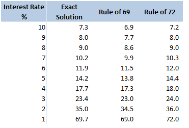
$$ln \left( 1 + \frac{i}{100} \right) = \frac{r}{100} – \frac{r^2}{20000} + … $$
In our case, it is more convenient to write this as:
$$ln \left( 1 + \frac{i}{100} \right) = \frac{1}{100} \left( r – \frac{r^2}{200} + … \right) $$
For $r<10$, the second term is less than $\frac{100}{200} = 0.5$. Given the first term is of the order $10$, this means we are only throwing out an adjustment of less than $5 \%$ to our final answer.

Taking just the first term of the Taylor expansion, we end up with:
$$n \approx \frac{69.3 \%}{\frac{1}{100} * \frac{1}{r}}$$
And rearranging gives:
$$n \approx \frac{69.3}{r}$$
So we see, we are pretty close to $ n \approx \frac{72}{r}$.
​
Why 72?

We saw above that using just the first term of the Taylor Expansion suggests we should be using the ‘rule of 69.3%' instead. Why then is this the rule of 72?
​
There are two main reasons, the first is that for most of the interest rates we are interested in, the Rule of 72 actually gives a better approximation to the exact solution, the following table compares the exact solution, the approximation given by the ‘Rule of 69’, and the approximation given by the Rule of 72:

The reason for this is that for interest rates in the 4%-10% range, the second term of the Taylor expansion is not completely negligible, and act to make the denominator slightly smaller and hence the fraction slightly bigger. It turns out 72 is quite a good fudge factor to account for this.
​
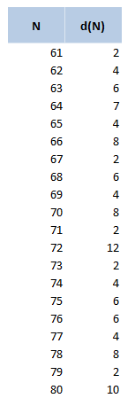
Another reason for using 72 over other close numbers is that 72 has a lot of divisors, in particular out of all the integers within 10 of 72, 72 has the most divisors. The following table displays the divisors function d(n), for values of n between 60 and 80. 72 clearly stands out as a good candidate.

​The rule of 72 in Actuarial Modelling

The main use I find for this trick is in mentally adjusting historic claims for claims inflation. I know that if I put in 6% claims inflation, my trended losses will double in size from their original level approximately every 12 years. Other uses include when analysing investment returns, thinking about the effects of monetary inflation, or it can even be useful when thinking about the effects of discounting.
​
Can we apply the Rule of 72 anywhere else?

As an aside, we should be careful when attempting to apply the rule of 72 over too long a time period. Say we are watching a movie set in 1940, can we use the Rule of 72 to estimate what values in the movie are equivalent to now? Let's set up an example and see why it doesn't really work in practice. Let's suppose an item in our movie costs 10 dollars.  First we need to pick an average inflation rate for the intervening period (something in the range of 3-4% is probably reasonable). We can then reason as follows; 1940 was 80 years ago, at 4% inflation, $\frac{72}{4} = 18$, and we’ve had approx. 4 lots of 18 years in that time. Therefore the price would have doubled 4 times, or will now be a factor of 16. Suggesting that 10 dollars in 1940 is now worth around 160 dollars in today's terms.

It turns out that this doesn’t really work though, let’s check it against another calculation. The average price of a new car in 1940 was around 800 dollars and the average price now is around 35k, which is a factor of 43.75, quite a bit higher than 16. The issue with using inflation figures like these over very long time periods, is for a given year the difference in the underlying goods is fairly small, therefore a simple percentage change in price is an appropriate measure. When we chain together a large number of annual changes, after a certain number of years, the underlying goods have almost completely changed from the first year to the last. For this reason, simply multiplying an inflation rate across decades completely ignores both improvements in the quality of goods over time, and changes in standards of living, so doesn't really convey the information that we are actually interested in.
​