As a rule of thumb, news outlets like the Guardian [1] or BBC News [2] don't typically report on the decisions of the Delaware Court of Chancery, a fairly niche 'court of equity' which decides matters of corporate law in the state of Delaware. That is of course, unless those decisions involve Elon Musk. Recently, the Delaware court handed down a judgement which voided a /$56bn pay-out which was due to Musk for his role as Tesla’s CEO. The reasoning behind striking it down is quite legal and technical, and not really my area of expertise but Matt Levine has a good write up for those interested. [3]

What I am interested in is thinking about how we would assess the fairness of the pay-out. Now fairness is a slippery concept, but I'm going to present one angle, which I've haven't seen discussed elsewhere yet, which I think is one possible way of framing the situation.

Investopedia defines TBVPS to be:

"Tangible book value per share (TBVPS) is the value of a company’s tangible assets divided by its current outstanding shares." [1]

I'm pretty sure this is incorrect. or at best misleading!

I wrote a python script which uses Selenium to scrape the predictions for Fed rate movements from the CME FedWatch tool.

www.cmegroup.com/trading/interest-rates/countdown-to-fomc.html#resources

The tool works by converting the price of a 30 day Fed Fund future into an implied probability of a given range of yields.

The CME website embeds the output in a something called an 'iframe', which I had never heard of before, and the iframe then contains a dashboard powered by something called Quikstrike. It took me a while to figure out how to switch focus to the iframe, as you can't simply reference elements inside the iframe without first switching focus.

The script below may not look too complicated, but believe me, it took a while to write.

Old Federal Reserve building Philadelphia, Source: https://commons.wikimedia.org/wiki/User:Beyond_My_Ken

Financial Year 2020 results have now been released for the top 5 reinsurers and on the face of it, they don’t make pretty reading. The top 5 reinsurers all exceeded 100% combined ratio, i.e. lost money this year on an underwriting basis. Yet much of the commentary has been fairly upbeat. Commentators have downplayed the top line result, and have instead focused on an ‘as-if’ position, how companies performed ex-Covid.
​
We’ve had comments like the following, (anonymised because I don’t want to look like I’m picking on particular companies):

"Excluding the impact of Covid-19, [Company X] delivers a very strong operating capital generation"

“In the pandemic year 2020 [Company Y] achieved a very good result, thereby again demonstrating its superb risk-carrying capacity and its broad diversification.”

Obviously CEOs are going to do what CEOs naturally do - talk up their company, focus on the positives - but is there any merit in looking at an ex-Covid position, or is this a red herring and should we instead be focusing strictly on the incl-Covid results?

I actually think there is a middle ground we can take which tries to balance both perspectives, and I’ll elaborate that method below.

I'm always begrudgingly impressed by brokers and underwriters who can do most of their job without resorting to computers or a calculator. If you give them a gross premium for a layer, they can reel off gross and net rates on line, the implied loss cost, and give you an estimate of the price for a higher layer using an ILF in their head. When I'm working, so much actuarial modelling requires a computer (sampling from probability distributions, Monte Carlo methods, etc.) that just to give any answer at all I need to fire up Excel and make a Spreadsheet. So anytime there's a chance to do some shortcuts I'm always all for it!

One mental calculation trick which is quite useful when working with compound interest is called the Rule of 72. It states that for interest rate $i$, under growth from annual compound interest, it takes approximately $\frac{72}{i} $ years for a given value to double in size.

Why does it work?

Here is a quick derivation showing why this works, all we need is to manipulate the exact solution with logarithms and then play around with the Taylor expansion.

We are interested in the following identity, which gives the exact value of $n$ for which an investment doubles under compound interest:
$$ \left( 1 + \frac{i}{100} \right)^n = 2$$
Taking logs of both sides gives the following:
$$ ln \left( 1 + \frac{i}{100} \right)^n = ln(2)$$
And then bringing down the $n$:
$$n* ln \left( 1 + \frac{i}{100} \right) = ln(2)$$
And finally solving for $n$:
$$n = \frac {ln(2)} { ln \left( 1 + \frac{i}{100} \right) }$$
So the above gives us a formula for $n$, the number of years. We now need to come up with a simple approximation to this function, and we do so by examining the Taylor expansion denominator of the right have side:

We can compute the value of $ln(2)$:

The Taylor expansion of the denominator is:
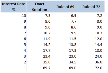
$$ln \left( 1 + \frac{i}{100} \right) = \frac{r}{100} – \frac{r^2}{20000} + … $$
In our case, it is more convenient to write this as:
$$ln \left( 1 + \frac{i}{100} \right) = \frac{1}{100} \left( r – \frac{r^2}{200} + … \right) $$
For $r<10$, the second term is less than $\frac{100}{200} = 0.5$. Given the first term is of the order $10$, this means we are only throwing out an adjustment of less than $5 \%$ to our final answer.

Taking just the first term of the Taylor expansion, we end up with:
$$n \approx \frac{69.3 \%}{\frac{1}{100} * \frac{1}{r}}$$
And rearranging gives:
$$n \approx \frac{69.3}{r}$$
So we see, we are pretty close to $ n \approx \frac{72}{r}$.
​
Why 72?

We saw above that using just the first term of the Taylor Expansion suggests we should be using the ‘rule of 69.3%' instead. Why then is this the rule of 72?
​
There are two main reasons, the first is that for most of the interest rates we are interested in, the Rule of 72 actually gives a better approximation to the exact solution, the following table compares the exact solution, the approximation given by the ‘Rule of 69’, and the approximation given by the Rule of 72:

The reason for this is that for interest rates in the 4%-10% range, the second term of the Taylor expansion is not completely negligible, and act to make the denominator slightly smaller and hence the fraction slightly bigger. It turns out 72 is quite a good fudge factor to account for this.
​
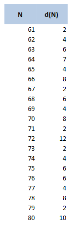
Another reason for using 72 over other close numbers is that 72 has a lot of divisors, in particular out of all the integers within 10 of 72, 72 has the most divisors. The following table displays the divisors function d(n), for values of n between 60 and 80. 72 clearly stands out as a good candidate.

​The rule of 72 in Actuarial Modelling

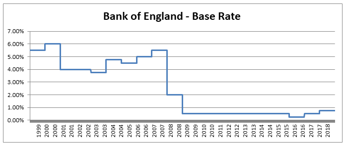
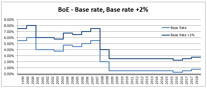
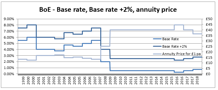
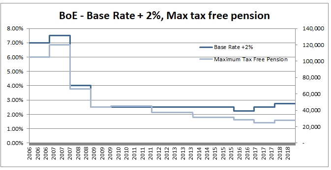
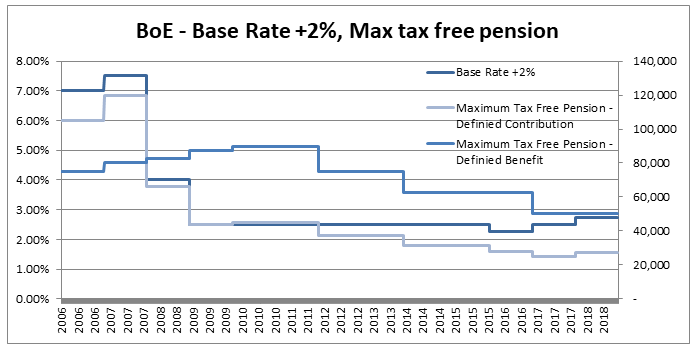
The main use I find for this trick is in mentally adjusting historic claims for claims inflation. I know that if I put in 6% claims inflation, my trended losses will double in size from their original level approximately every 12 years. Other uses include when analysing investment returns, thinking about the effects of monetary inflation, or it can even be useful when thinking about the effects of discounting.
​
Can we apply the Rule of 72 anywhere else?

As an aside, we should be careful when attempting to apply the rule of 72 over too long a time period. Say we are watching a movie set in 1940, can we use the Rule of 72 to estimate what values in the movie are equivalent to now? Let's set up an example and see why it doesn't really work in practice. Let's suppose an item in our movie costs 10 dollars.  First we need to pick an average inflation rate for the intervening period (something in the range of 3-4% is probably reasonable). We can then reason as follows; 1940 was 80 years ago, at 4% inflation, $\frac{72}{4} = 18$, and we’ve had approx. 4 lots of 18 years in that time. Therefore the price would have doubled 4 times, or will now be a factor of 16. Suggesting that 10 dollars in 1940 is now worth around 160 dollars in today's terms.

It turns out that this doesn’t really work though, let’s check it against another calculation. The average price of a new car in 1940 was around 800 dollars and the average price now is around 35k, which is a factor of 43.75, quite a bit higher than 16. The issue with using inflation figures like these over very long time periods, is for a given year the difference in the underlying goods is fairly small, therefore a simple percentage change in price is an appropriate measure. When we chain together a large number of annual changes, after a certain number of years, the underlying goods have almost completely changed from the first year to the last. For this reason, simply multiplying an inflation rate across decades completely ignores both improvements in the quality of goods over time, and changes in standards of living, so doesn't really convey the information that we are actually interested in.
​

Pensions and tax you think to yourself - he’s managed to find the two most boring subjects possible and now he appears to be planning to write about a combination of them! Is this some sort of attempt to win an award for the most boring and tedious blog post every?

Well what if I told you this blog post, whilst being about pension and tax was also about a burning social justice, about high finance, and about death? Would you find that interesting? 

Okay, so I may got slightly carried away in that last paragraph and over sold slightly. This is less of a 'burning social injustice', and more an 'unfair outcome' which happens to only affect people who are already well off - but someone has to write about this stuff right? And the current status quo is genuinely unfair I promise.

Lifetime Allowance

​Before diving into the unfairness I mentioned earlier, we need to briefly set the scene. Let’s think about all the types of tax that the government levies on us; we get taxed on our income (income tax), we get taxed on our property wealth (council tax), we get taxed on our wealth when we die (inheritance tax), and we get taxed when we buy things (VAT and other sales taxes). Since the government taxes just about every financial transaction we make, they can tweak all these different types of tax to incentivise and disincentivizes certain behaviours. One thing governments have traditionally been very keen on incentivising is getting its citizens saving enough for retirement. The way this has historically been done is to allow income tax relief on the proportion of an employee’s gross salary which is put into a pension. i.e. If you earn £30,000 and put £5,000 of that into a pension, then you pay no tax on the £5,000 and are then taxed as if you only earn £25,000.
​
You might think to yourself great, so now people are saving more for their retirement and everyone lives happily ever after, the end. Well not quite. The problem with this arrangement is certain unscrupulous individuals started to use this mechanism to avoid paying tax. Let’s say you’re 64, quite well off, and hoping to retire next year, why not chuck most of your money into your pension? You can live off your savings for a year and then all that money you would have taken as income and therefore been taxed on can instead be deferred for a year, taken as pension when you retire, and you would pay no income tax on that year's salary. Or let’s suppose an individual come from a very wealthy family, and doesn't really need to get paid a salary to live on, then they could just put their entire salary into a pension, not take anything until they retire (at 55), and then not pay any tax at all on their earnings from their job across their entire career.

Okay, fine, it sounds like we’re going to need some caps on the maximum pension tax relief to stop people doing this. Let’s say – £225k per annum is the maximum that can be put into a pension pot per year, and £1.5m is the total size of a pension pot you can build up before we start making people pay tax. That’s a large amount of money, who’s going to complain about that?

These were the levels set by Tony Blair’s government between 2004 and 2006. These caps were then slowly increased over time, reaching a height of around £250k pa, and £1.8m as a lifetime allowance in 2011. These are very big figures, and it’s hard to imagine anyone objecting to a tax on an annual pension contribution above £250k.

In 2011, with a rapidly expanding budget deficit to deal with and a promise to balance the books, the Conservative government instigated their infamous austerity programme. The tories had pledged to ring-fence certain areas of government spending (the NHS, and Education for example), they therefore started to look around for other areas to raise additional income which had not traditionally been taped. Tax relief for high earners seemed like an obvious target, and who can really say that the rich should not have to pay additional tax given the situation to help try to protect spending on areas such as policing or social care.

By 2014 the annual allowance (the amount that can be saved per annum) had been reduced to £40k per annum, and the lifetime allowance was down to £1m. These values still seem high, however with the economy in the state it was, they are perhaps not as high as they first appear. This reduction came during a period of all-time low interest rates, I'm going to demonstrate which this caused issued by examining a series of graphs.

The following graph displays the Bank of England base rate for the last twenty years, notice the significant reduction in 2007 following the global financial crisis. Note we have been at this very low level ever since.

As a proxy for the investment return a pension or life insurance company could receive on a long term almost risk-free investment I’m going to use Base rate + 2%, I've plotted this as well on the graph below:

Okay, so why is this important?

The interesting idea is that the ‘price’ of an annuity can be approximated using quite a simple formula. It is (very) roughly equal to:

$ A = \frac{1}{i} $

Where i is our investment return.

What does this mean in real numbers? If I want to retire and get a pension of £10,000 per annum, Then the price of that is going to be 10,000 * A = 10,000 / i. If i=10%, then I will need to have a pot of £100,000. If i = 1%, then I will need a pot of £1m.
​
Let’s plot the implied annuity price on the same chart as a secondary axis:

So we see we have this reciprocal relationship, as interest rates go down, the cost of an annuity goes up. At the moment, due to the very low interest rates, it costs something like £37 to purchase an annuity of £1 per annum for life.

Interesting you might (or might not) think. But this annuity price becomes useful if we combine it with the lifetime tax-free allowance. If we assume a potential retiree is going to use their pension pot to purchase an annuity, then to calculate the level of pension they will be able to get, we need to take their pension pot and divide by the cost of the annuity.

The graph below shows the approximate tax-free pension one could expect if retiring with a pension pot equal to the full Lifetime allowance, using the prevailing annuity rates which are in turn based on the prevailing interest rates.
​

So we see that through a combination of the LTA being reduced significantly and interest rates bottoming out, we are now in the position where the maximum tax-free pension (based on approximate annuity rates) is as little as £25k. A far cry from the approximately £100k when the rule was first implemented.

What about that burning social injustice you mentioned?

​But at least we are all treated the same right? Well not exactly… all of the above glossed over one quite important point, it assumes that the individual in question has a defined contribution pension. For individuals with a final salary pension (which includes MPs, Judges, a majority of CEOs and senior public sector employees), the LTA is calculated with reference to a fixed annuity factor of 20. Given the actual average annuity price is more like 40, this has a massive impact. Let’s plot this on a graph as well.

​

Hmmm, so we see that in 2006 when the LTA was first set up, this factor of 20 was quite generous to Defined Contribution pension holders, they could often retire with a pension of around £120k without paying any tax, whereas a defined benefit pension holder could only retire with a maximum of approx. £80k. This has now flipped, due to changes in annuity rates, and the fact that this factor has not been adjusted for so long. Under current conditions, the maximum pension that can be taken tax free is around £25k pa for a definied contribution pension, but around £50k pa for a definied benefit pension. 

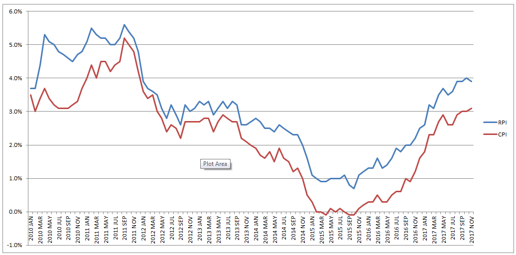
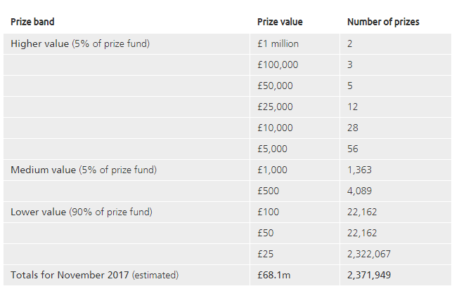
So what is the point of all this? What am I advocating?

To me it seems clear that we need (approximate) equality of outcome in terms of taxation for defined contribution pensions compared to defined benefit schemes. This could be achieved in one of two ways, either we apply some sort of floor to how low the tax free pension can reduced to for defined contribution pensions, or we adjust the defined benefit annuity factor  periodically to keep it roughly in line with market conditions and therefore apply a lower maximum tax free rate to defined benefit pensioners. This would correct the current system by which judges and MPs (and other people with DB pensions) get significant tax breaks at retirement compared to individuals with DC pensions.

Last week it was announced that UK Rail Fares were to increase once again at the maximum allowed rate - 3.4%, corresponding to the RPI increase in July 2017.

News article:
​www.bbc.co.uk/news/business-42234488

When reading this it got me thinking - why is RPI even being used any more? Aren't we supposed to be using CPI now?

In 2013 the ONS stated that:

"Following a consultation on options for improving the Retail Prices Index (RPI), the National Statistician, Jil Matheson, has concluded that the formula used to produce the RPI does not meet international standards and recommended that a new index be published."

So basically the ONS no longer endorses RPI as the best indicator of the level of inflation in the economy. The ONS instead supports the use of CPI. So why does it matter that some organisations are still using RPI?  To see why, let's take a look at a chart showing the historic RPI and CPI increases in the UK:

Source:
www.ons.gov.uk/economy/inflationandpriceindices

RPI has been greater than CPI in every single month since 2010. In fact, in this time period, RPI has been an average of 0.8% higher than CPI. This fact might go some way to explain why the Government is so slow to move rail increases from RPI to CPI. This way the Government and Rail Companies can claim that they are only increasing their costs in line with inflation, which seems fair, yet the index they are using is actually higher than the usual inflation index used in the UK.

The Government also indexes some of it's outgoings by an inflation index, for example the State Pension, so at least this is also being consistently overstated right?

Well actually no! Wherever the government is using an inflation index to increase payments, it seems to have already transitioned to a CPI increase. Let's look at the list of items which use the inflation index which is more beneficial to the Government: (remember that CPI is almost always lower than RPI):

There are some pretty hefty items on the list, including, the State Pension, Benefit Payments, Rail Fares,  Utility bills, Student Loans. The ones that decrease government spending seem to have already transitioned over, and the ones that increase the amount of tax collected, or the cost of regulated items all seem to still be using the higher RPI index.

Now let's look at the list of items which use the inflation index which is to the disadvantage of the Government.

I've got to admit, up until recently, I never really understood why anyone would buy Premium Bonds. You get an expected return of 1.15%, which is well below other asset classes, there is significant volatility in returns, and the 1.15% is not even guaranteed, i.e. it's possible you'll never get any returns at all. The risk and return profile just seem completely out of sync with the alternatives. But after speaking to my Grandad about them yesterday, I started to understand why some of the soft factors make them so attractive to savers. Then when I was mulling over it further, I realised that these soft factors would actually be seen as negatives when viewed through the lens of Modern Portfolio Theory.

What are Premium Bonds?

Premium Bonds were introduced by Harold Macmillan in 1956 in an attempt to encourage individuals to save more, and also to help raise money to finance Government spending. The bonds pay out prizes to bondholders based on a lottery system and are organised by the National Saving and Investment Agency. The Government uses the money to help finance the Public Sector Borrowing Requirement (the difference between the amount of tax the Government collects .every year, and the amount the Government spends - which has been negative for about 30 years now!)

Every month, the NSI distributes a prize pool randomly among Bond holders, the pool is  calculated so that the total annual amount paid out is equivalent to 1.15% of the total value of bonds held over the year. So as there are approximately £71bn of bonds owned in total, the prize pool will be £71bn * 1.15% = £817m per year, or £68.1m per month. This £68.1 million will then be distributed randomly to bond owners in various sized prices using the following table:

Both the interest rate used to calculate the overall prize pool, and the distribution of prizes is updated from time to time, to account for changes in the overall market conditions. This table is correct as at the date of this post.

Advantages of Premium Bonds

In spite of their relatively low rate of return, Premium Bonds do a have a number of features that make them attractive to individual savers:

• The scheme is 100% guaranteed by HMRC
• There is no risk to the capital invested
• The Scheme is relatively easy to understand
• Investors have immediate access to capital without penalties or delays if they wish to withdraw money
• There is a low minimum investment (£100 for new investors, £50 for current holders)
• Income from Premium Bonds is tax free
• There is a possibility of winning a £1 million payout

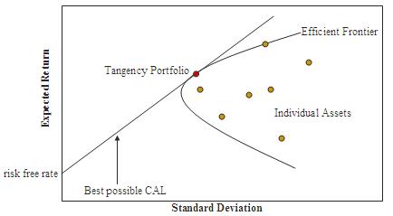
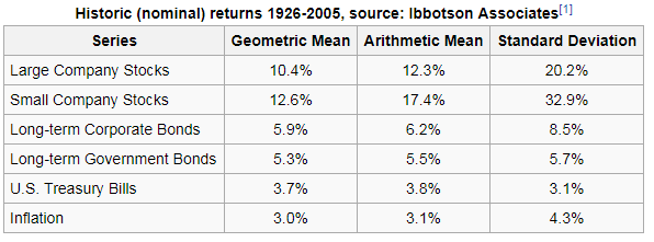
For many individual investors, the first five bullet points are extremely important. I think many savers would even say that are necessary requirements to get them to invest their money.

It's the final bullet point which is particularly interesting though, the possibility of winning £1 million is a big selling point of Premium Bonds. This should interest any analyst who uses conventional theories of investment, as most investment theories would consider this a downside of Premium Bonds. To understand why this is the case, we'll need to take a brief look at Modern Portfolio Theory.

Volatility of Investment Returns as a Risk Measure

All the possible investment classes have different risk and return profiles. Some provide high returns, but also contain high levels of risk. Others offer lower levels of return, but also come with less risk. In order to compare different investment classes in a consistent way, we need a single definition of risk and return which we can then apply to each class. The obvious measure to use for return is simply the Mean Expected Return. The situation isn't so straight forward for our risk measure though. There is no perfect measure of risk, and all the possible measures have advantages and disadvantages. In practice, the most commonly used measure is variance of return and this is the approach used in Modern Portfolio Theory:
en.wikipedia.org/wiki/Modern_portfolio_theory

Under Modern Portfolio Theory, we calculate the expected return of each investment class, along with the variance of return and plot this on a graph. An investor is then assumed to want to maximise the expected return, while minimising the variance of returns (because this corresponds to risk). This allows us to construct an 'efficient frontier' corresponding to those investments, which for a given return, minimise the risk. The following graph demonstrates this analysis.

By including the possibility of winning a £1 million prize, we are massively increasing the variance of the investment returns, but since the overall return is calibrated to a 1.15% expected return, the risk-reward profile of premium bonds (using variance as our measure of risk) looks terrible.

So we end up with the strange situation that one of the main selling points of Premium Bonds - the possibility of winning a £1 million prize each month, actually should make the investment less attractive under most theories of investment.

I did a quick calculation of the variance of returns provided by premium bonds, and it comes out at a whopping 35,000%. Most of this volatility is coming from the fact that two of the prizes are for £1 million, if we take out all the prizes above £1000 and reallocate the money to the smaller prizes the volatility reduces by about 400 times, down to around 90%. But even this is still considered very volatile compared to most investment classes. For example, Burton Malkiel in A Random Walk Down Wall Street provides the following table of historic asset class returns with accompanying volatility (which I then copied from Wikipedia)

So for comparison, we see that according to this analysis, investing in Small Companies Stocks provided an average return of 12.6%, much higher than premium bonds, yet only had a Standard Deviation of return of 32.9%.

Under the assumptions of Modern Portfolio Theory, by using variance of investment returns as a risk measure, we would conclude that investors would prefer not to have the possibility of the £1 million prize, but instead would prefer to have more smaller prizes included in the payout. This is clearly not the case.

Disadvantages of investing in Premium Bonds

So far we've talked about the advantages of investing in Premium Bonds, and we've also talked about how some of these selling points go against the conclusions of Modern Portfolio Theory (though I think this might say more about the state of Modern Portfolio Theory than Premium Bonds). Are there however any clear disadvantages to investing in Premium Bonds? I think there are, and here are a few of them:

• Premium Bonds do not give 'real' returns

We often distinguish between real and nominal investment returns when analysing investment classes. What this means is that some investment classes provide returns which are expected to be above inflation, other classes provide returns which are of a fixed amount and may be greater than or smaller than the level of inflation in the economy, these are called nominal returns.

To see what we mean by this, let's say you invest £1,000 in premium bonds in a given year and you get £25 in prizes, leaving you with £1,025 at the end of the year. Let's assume  also that prices (i.e. inflation) went up by 5% during the year, which means that in order to buy something which would have cost £1,000 at the start of the year, you would now need £1,050. So your £1,025 which you got back from the Premium Bonds at the end of the year, can now buy less than the £1,000 you put in originally. So that even though you've now got more money, the real return on your investment was negative.

Premium Bonds are currently paying out at 1.15%, whereas inflation in July 2017 was 2.6% according to the Office of National Statistics. This means that you are in effect losing money by holding Premium Bonds.

• There is no guarantee of returns

Due to the lottery structure of Premium Bond returns, it's possible (and in fact highly likely unless you hold large quantities of bonds) that you will get no investment returns at all.
For example, someone who holds £100 of Premium bonds has a 96% chance of not getting any prizes at all in a given year. This is in contrast to a fixed interest bank account, for example if it guarantee to pay 3% pa there would be no possibility of winning a £1 million prize, but which you could be certain would always give you your 3% return at the end of the year. If you are willing to go through the hassle of shopping around for a savings account which does guarantee 3%, then you'd probably be better off from a financial perspective investing in the savings account and then buying yourself a lottery ticket every week rather than investing in premium bonds.

• Low overall Investment returns

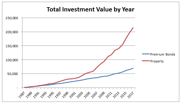
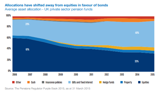
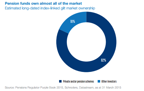
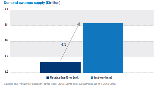
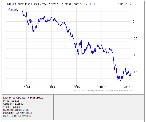
The expected return from Premium Bonds is much lower than the returns we could expect from other investment classes. To see how much of a different this can make, let's take two hypothetical savers, both of whom have been saving £100 per month ​for the last 30 years, one has been investing in Premium Bonds (and getting an average return of 3.5% pa) and another has been investing in a Property Fund (and getting a 10% average return). Over the years, the difference between these two expected returns can have a significant impact on the overall amount that they save. I ran a quick simulation of this with some volatility producing the following graph:

So we've talked about the positives and negatives of Premium Bonds, and also touched on
some inconsistencies between the marketing of Premium Bonds, and how they would be viewed using traditional finance techniques. Are there any other features of Premium  Bonds which are interesting? 

One quirk of Premium Bonds which seems to have captured people's imaginations is ERNIE. So who is ERNIE?

E.R.N.I.E

ERNIE stands for Electronic Random Number Indicator Equipment, and is the name of the machine that is used to randomly select which bonds win,

Due to the fact that Premium Bonds were first set up in 1957, creating a computer to generate random numbers was a non-trivial problem at the time. ERNIE was developed in the Post Office Research Station in North West London. 
​​

Despite its quaint sounding name, the Post Office Research Station was actually at the forefront of computing research during the 40s and 50s. The Colossus, the world's first electronic programmable computer, which had been developed during the second World War to help break one of the codes used by the Axis was developed at the Post Office Research Station. The details of Colossus were classified until the 1970s so it had limited impact on most other computers built around in the 50s and 60s, however the design of ERNIE was heavily influenced by the work that had been done on Colossus during the war as the same design team worked on both.

Unlike most computers today that are pseudo-random number generators, ERNIE was a true random number generator. It contained neon tubes, through which an electric current was passed. Due to the electrons bumping into the neon atoms as they passed through  the neon tube, the current leaving the neon tube varied randomly. This randomness was due to millions of tiny interactions between the electrons and the neon tube and was a source of true statistical randomness. This randomness was then calibrated so that ERNIE would select a collection of random numbers between 1 and 100 million, which corresponded to the Premium Bond numbers that people had purchased.

I struggled to follow a lot of the technical details of how ERNIE works, due to an insufficient knowledge of electrical engineering, but if you are interested the following link contains a technical document describing how ERNIE selected random numbers:
www.tnmoc.org/sites/default/files/Ernie-technology.pdf

I might do some reading up on Electrical Engineering at some point, and then write up exactly how ERNIE worked, because I couldn't find a decent non-technical description online.

Conclusion

Premium Bonds were a massive success when they were launched. They managed to get people excited about saving, and they gave the Government a cheap source of borrowing. I think it's a shame they have fallen by the wayside in recent years.

They are conceptually simple, they offer a lot of the guarantees that savers look for in an investment opportunity - protecting their capital, not locking them in for a fixed period - they exploit the popularity of lotteries in a positive way (by tricking people into saving more in order to play), and they don't require complicated decisions to be made by savers (who has time to trawl through the bewildering array of different options currently available - Cash ISAs, Stocks and Shares ISAs, NSI bonds, Fixed interest bank accounts....)
​
All too often, it seems Government savings schemes are designed by individuals steeped in financial theory who are too far removed from the savers who will be using the products. We should rethink how we design the kind of products offered by the NS&I and take more account of Behavioural Economics, and Marketing Strategies rather than relying on microeconomic models which assume rational investors, or relying on models of investment returns like Modern Portfolio Theory.

What even are Ogden Rates anyway?

The Ogden tables are tables of annuity factors, published by the Government's Actuary Department, which are used to calculate court awards for claimants who have had life changing injuries or a fatal accident and are eligible for a payout from their insurance policy.

For example, consider a 50 year old, male, primary school teacher who suffers a car accident which means that they will not be able to work for the rest of their life. The Ogden Tables will be used to calculate how much they should be paid now to compensate them for their loss of earnings. Suppose the teacher is earning a salary of £33,000 when they have the accident, then under the Ogden Rates prior to March 2017, the teacher would be paid a lump sum of £33,000* 20.53 = £677,490 where 20.53 is the factor from the tables.

How did the Government's Actuary Department come up with these factors?

The factors in the table are based on two main pieces of information, how long the person is expected to live, and how much money they can earn from the lump sum once they are given it (called the discount rate). It's this second part which has caused all the problems between the Ministry of Justice and the Insurance Industry.

The discount rate should be selected to match the return generated on assets. For example, if the claimant puts all their money in shares then on average, they will generate much more income than if they put the lump sum in a savings account.  So what should we assume our school teacher will invest their lump sum in? Since the school teacher will not be able to work again, and therefore will need to live off this money for the rest of their life, they will not want to risk losing all their money by investing in something too risky. In technical terms, we would say that the claimant is a risk adverse investor.

In order to mimic the investment style of this risk adverse investor, when the Ogden tables were first set, it was decided to assume that the investor would put all their money in index-linked bonds. There are a couple of reasons to assume this, many risk adverse institutional investors do purchase a lot of index-linked bonds, and also, the average discount rate for these bonds is readily available as it is already published by the UK DMO.

At the time the tables were set up, this seemed like a great idea, but recently it has made a lot of people very angry and been widely regarded as a bad move.

What are Index-linked bonds again?

In the 1981 the UK government started issuing a series of gilts which instead of paying a fixed coupon, paid a floating coupon which was a fixed percentage above the rate of inflation.

The UK Debt Management Office is responsible for issuing these bonds, and the following website has details of the bonds that are currently in issue. It's quite interesting to see how it all works:

www.dmo.gov.uk/reportView.aspx?rptCode=D1D&rptName=50545854&reportpage=D1D

The basic principle is if you purchase a bond that pays 2% coupons, if inflation is 3%, they would pay 3%+2%, if inflation was 5%, then they would pay 5% + 2%. Due to the fact that these bonds always gave a fixed real return (2% in this case), institutional investors really like them. Because there is no inflation risk, on average index-linked bonds cost more than fixed coupon bonds once you account for the effects of inflation. Pension Schemes in particular purchase a lot of these bonds, 

Why do Pension Schemes like these bonds so much?

Most pensions are increased annually in line with inflation, due to this Pension Schemes like to hold assets that also go up in line with inflation every year. In order to get real returns on their investments, Pension Schemes traditionally held a mix of shares and index-linked bonds, the shares gave better returns, but the bonds were more safe.

This all started to go very wrong after the financial crisis . A huge drop in interest rates and investment returns, combined with soaring life expectancy lead to more and more pension schemes winding up and the remaining ones have funding issues. As the schemes started winding up they became more and more risk adverse and started to move away from the more volatile assets like shares and moved towards index-linked bonds instead.

This table from the PPF's Purple Book shows the move away from shares into bonds.

We can see that back in 2006, prior to the financial crisis, Pension Schemes were on average holding around 61% of their assets in equities. When we look again at 2014 this percentage has dropped to 33% and the slack has largely been taken up by bonds.

Pension Schemes like these assets so much in fact that Schroders estimated that 80% of the long term index-linked gilts market is held by private sector pension schemes as the following chart shows.

Source:
www.schroders.co.uk/en/SysGlobalAssets/schroders/sites/ukpensions/pdfs/2016-06-pension-schemes-and-index-linked-gilts.pdf​
​

As you might expect with such a disparity between supply and demand, ​Pension funds have been chasing these assets so much that yields have actually become negative. This means that Pension Schemes on average are paying the government to hold their money for them, as long as it's protected against inflation.

Here is a chart showing the yield over the last 5 years for a 1.25% 2032 index-linked gilt.

Source:
www.fixedincomeinvestor.co.uk/x/bondchart.html?id=3473&stash=F67129F0&groupid=3530

So what does this have to do with Ogden Rates?

So now we are in a position to link this back to the recent change in the Ogden Rate.

Because the yield on index-linked bonds has traditionally been used as a proxy for a risk-free real return, the yield is still used to decide the discount rate that should be used to calculate court award payouts.

Because Pension Schemes have been driving up the price of these bonds so much, we have the bizarre situation that the amount that insurance companies have to pay out to claimants has suddenly jumped up considerably. In the case of a 20 year old female for example, the amount that would be paid out has almost tripled. As these pay outs are already considerable, the financial impact of this change has been massive.

So what should the Government do?

There is no easy answer, if the Government doesn't use the yield on index-linked gilts to calculate the Ogden rate then there is no obvious alternative. I think the most reasonable alternative would be to use a weighted average of returns on the types of assets that an average claimant would hold. For example, we might assume the claimant is going to hold 50% of their lump sum in cash, 30% in shares, and 20% in bonds, and we would then calculate the weighted return from this portfolio.

The issues with doing nothing is that the additional cost from these increased pay outs will inevitably be passed on to the policyholders through higher premiums. So ultimately there is an issue of fairness whereby people who are receiving payouts are being paid a disproportionate amount of money, and this is being subsidised by policyholders other policyholders.

If people could live forever, then would they still be able to retire or would pension schemes become bankrupt from having to pay out never ending streams of money to eternally youthful pensioners?
 
This might sound like an overly academic question, however I've noticed a glut of articles recently about the prospects of substantially extending the human lifespan, for example:
 
http://gizmodo.com/peter-thiel-is-right-about-one-thing-1785104345
 
And a feature in this week's economist:
 
http://www.economist.com/news/leaders/21704791-science-getting-grips-ways-slow-ageing-rejoice-long-side-effects-can-be
 
Many of these articles raise the point that extending the human lifespan would have an effect on the affordability of retirement. Claiming that retirement as we know it would come to an end.
 
Is this correct though? Most of the articles that I found simply state that retirement would now be impossible without explaining precisely why. I thought I'd do some calculations and see how much of an effect increased lifespans would have on pension scheme funding, It turns out that the situation is not as bad as it seems.
 
First we need to introduce an actuarial technique that allows us to calculate the cost of paying someone a pension into the future.

Perpetuity

​Suppose that we have a payment stream of amount $£1$, payable annually, and paid forever. Graphically we are talking about the following situation::

​ 

​Can we place a value on this series of payments?
 
You might suppose that since we are paying out an infinite amount of money that the value of the perpetuity (which is the name of a payment stream that continues indefinitely) should be infinite.
 
However finance uses a concept called ‘net present value’ or NPV, to assign a value to this stream, and this value turns out to be finite.
 
Time value of money

First we need some extra information, let's assume that we have access to a risk-free bank account that pays out an interest rate of $i$% per annum. (For example, $i$ might be $5$). So that if we invest $1$ at time $t=0$, it will be worth $1*(1+i)$ at time $t=1$, and worth $1*(1+i)*(1+i)$ at time $t=2$.
 
Let's first solve a simplified problem and just consider the value of the first payment of $1$ at time $1$. If we wish to invest an amount of money now, so that we can pay the $1$ due at time $t = 1$ with the money we have invested, then if we put $1*(1+i)^{-1}$ in the bank account now, this will be worth $1$ at time $1$. Similarly to invest an amount now so that we will be able to pay the amount $1$ at time $n$, we need to invest ${1/(1+i)}^{-n}.$
 
Going back to the original problem, we can use this result to calculate the amount we should invest now so that we can pay all the future payments. It will be:
 
$\sum_{k=1}^{\infty} {1/(1+i)}^{-k} $ 

This is just a geometric series, which sums to $1/ (1- (1+i)) = 1/i.$
​
Therefore the amount we need to invest is $1/i$. So, if $i=5%$ as we had earlier, then we  actually only need to invest $20$ now in order to pay able to pay someone $1$ every year, for ever!
 
Checking the Result
 
Let's check that this makes sense. Suppose that we do invest this amount at $t=0$, then at $t=1$ we will have $(20)(1.05) = 1 + 20$.
 
Which gives us $1$ to pay the perpetuity, and leaves enough to invest the original amount again. We can see that if nothing else changes, this system can continue indefinitely.
 
Returning to our previous question, would it be possible to pay a pension to someone who will live forever? The answer is yes. We can even calculate the amount that we would need to invest now to pay the pension.
 
Increasing pensions
 
This system we have derived is not very realistic though. Most pensions increase over time, for example the state pension in the UK increases by the minimum of CPI, $2.5%$ and the average annual wage growth. Given that a pension that increases over time will not just pay out an infinite amount, but will also grow to be infinitely big. Would such a pension still work in a scenario where pensioners live forever?
 
It turns out in fact that yes, such a system is still sustainable under certain conditions.
 
Let’s suppose that our perpetuity increases at a rate of $g%$ per year, so here we might assume that $g=2.5$. Then if we derive the amount that we will need to invest now (at an investment rate of $i%$) we find that we will need $((1+g)/(1+i))^n$. Summing all of these values gives the following initial value:
 
$\sum_{k=1}^{\infty} {(1+g)/(1+i)}^{-k} $this is another geometric sum, however now we need to consider convergence, this sum will converge iff $((1+g)*(1+i)) <1$. That is, the sum will converge iff we can find an investment that grows faster than the perpetuity we have promised to pay.
 
If the sum converges then it will converge to $(1/(i-g))$.
 
So using the example we had earlier, where $i=5%$, $g=2.5%$ we would need to invest $ 1/0.025 = 40$. Which is substantially more than the non-increasing annuity but still finite.
 
So we see that even when the pension is increasing, we can still afford to set it up.

Mortality Premium
 
Can’t we still make the argument that pensions will become unaffordable due to the fact that these perpetuities will still cost a lot more.
 
Let's compare the value of an annuity assuming the pensioner will live to the average life expectancy with one where the pensioner is assumed to live forever.

Looking in my orange tables (the name for the Formula and Tables for Actuarial Exams) I see that the cost of a non-increasing pension of $1$ per year, paid to a $65$ year old male at a discount rate of $4%$ is $12.66$. Compare this to the value of $25$ to pay the pension forever, we see that the cost of the pension is roughly double. This amount is much higher, but it's interesting to note that the increase in cost is similar as that between increasing and non-increasing pensions!

Can we actually live forever?

We should also consider the fact that mortality will never actually be $0$ even if ageing is eliminated. Presumably accidents, and possibly even illness unrelated to age would still exist and for this reason we would not expect to have to pay these pensions forever. If you live long enough, then the probability of all non-impossible events occurring at some point should eventually reach $1$. This means that eventually even the most unlikely accidents would eventually happen if you lived long enough. 
​

 In Options, Futures and Other Derivatives, Chapter 10, Hull derives lower bounds for option prices for European put and call options for dividend paying stocks.

The result in Hull:

For a call option:

​For a put option:

And he also derives upper bounds for European put and call options for non-dividend paying stocks.

For a call option:

​For a put option:

​But he doesn't derive upper bounds for European put and call options for dividend paying stocks. And for call options this gives us a tighter upper bound. Also I wasn't able to find this bound online for some reason, it's almost like everyone is just copying these results from other people and not actually deriving them themselves.

The new Result

I was working through Hull's Options, Futures and other Derivatives when Hull states that the price of a Bond paying semi annual coupons in line with six month LIBOR, and discounted using a six month LIBOR discount rate is par. To me this statement seems like it's probably true but I wasn't 100%. I couldn't find the proof online, but it turns out that it is true, here is my derivation.