Piketty also adds colour by tying his observations to the literature written at the time (Austen, Dumas, Balzac), and how the assumptions made by the authors around how money, income and capital work are also reflected in the economic data that Piketty obtained.
​
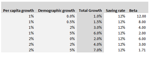
Hopefully I've convinced you Piketty's programme is a worthwhile one, but that still leaves the fundamental question - is his analysis correct? That's a much harder question to answer, and to be honest I really don't feel qualified to pass judgement on the entirety of the book, other than to say it strikes me as pretty convincing from the limited amount of time I've spent on it.

​In an attempt to contribute in some small way to the larger conversation around Piketty's work, I thought I'd write about one specific argument that Piketty makes that I found less convincing than other parts of the book. Around 120 pages in, Piketty introduces what he calls the ‘Second Fundamental Law of Capitalism’, and this is where I started having difficulties in following his argument.

The Second Fundamental Law of Capitalism

​​The rule is defined as follows: 
$$ B = \frac{s} { g} $$
Where $B$ , as in Piketty’s first fundamental rule, is defined as the ratio of Capital (the total stock of public and private wealth in the economy) to Income (NNP):
$$B = \frac{ \text{Capital}}{\text{Income}}$$

And where $g$ is the growth rate, and $s$ is the saving rate.
​
Unlike the first rule which is an accounting identity, and therefore true by definition, the second rule is only true ‘in the long run’. It is an equilibrium that the market will move to over time, and the following argument is given by Piketty:

“The argument is elementary. Let me illustrate it with an example. In concrete terms: if a country is saving 12 percent of its income every year, and if its initial capital stock is equal to six years of income, then the capital stock will grow at 2 percent a year, thus at exactly the same rate as national income, so that the capital/income ratio will remain stable.

By contrast, if the capital stock is less than six years of income, then a savings rate of 12 percent will cause the capital stock to grow at a rate greater than 2 percent a year and therefore faster than income, so that the capital/income ratio will increase until it attains its equilibrium level.

Conversely, if the capital stock is greater than six years of annual income, then a savings rate of 12 percent implies that capital is growing at less than 2 percent a year, so that the capital/income ratio cannot be maintained at that level and will therefore decrease until it reaches equilibrium.”

I’ve got to admit that this was the first part in the book where I really struggled to follow Piketty’s reasoning – possibly this was obvious to other people, but it wasn’t to me!

Analysis – what does he mean?

Before we get any further, let’s unpick exactly what Piketty means by all the terms in his formulation of the law:

Income = Net national product = Gross Net product *0.9
(where the factor of 0.9 is to account for depreciation of Capital)

$g$ = growth rate, but growth of what? Here it is specifically growth in income, so while this is not exactly the same as GDP growth it’s pretty close. If we assume net exports do not change, and the depreciation factor (0.9) is fixed, then the two will be equal.

$s$ = saving rate – by definition this is the ratio of additional capital divided by income. Since income here is net of depreciation, we are already subtracting capital depreciation from income and not including this in our saving rate.

Let’s play around with a few values, splitting growth $g$, into per capita growth and demographic growth we get the following. Note that Total growth is simply the sum of demographic and per capita growth, and Beta is calculated from the other values using the law.
​

​So why does Piketty introduce this law?

The argument that Piketty is intending to tease out from this equality is the following:

• Given per capita GDP is on average lower than many people realise (on the order of 1-2% pa in the long run)
• And given GDP growth is no longer offset by demographic GDP growth in many advanced economies, i.e. the demographic growth component is now very low
• GDP growth in the future is likely to only be on the order of 1.5% pa.
• Therefore for a fixed saving rate, and relatively low growth, we should expect much higher values of Beta than we have seen in the last 50 years.

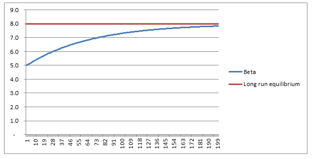
In fact using $g=1.5 \%$ as a long term average, we can expect Beta to crystallise around a Beta of $8$! Much higher than it has been for the past 100 years.

Analysis - convergence
​
As Piketty is quick to point out, this is a long run equilibrium towards which an economy will move. Moreover, it should be noted that the convergence of this process is incredibly slow.

Here is a graph plotting the evolution of Beta, from a starting point of 5, under the assumption of $g=1.5 \%$, $s = 12 \%$:

​So we see that after 30 years ( i.e. approx. one generation), Beta has only increased from its starting point of $5$ to around $6$, it then takes another generation and a half to get to $7$, which is still short of its long run equilibrium of $8$.

Analysis - Is this rule true?

Piketty is of course going to want to use his formula to say interesting things about the historic evolution of the Capital/Income ratio, and also use it to help predict future movements in Beta. I think this is where we start to push the boundaries of what we can easily reason, without first slowing down and methodically examining our implicit assumptions.

For example – is a fixed saving rate (independent of changes in both Beta, and Growth) reasonable? Remember that the saving rate here is a saving rate on net income. So that as Beta increases, we are already having to put more money into upkeep of our current level of capital, so that a fixed net saving rate is actually consistent with an increasing gross saving rate, not a fixed gross saving rate. An increasing gross saving rate might be a reasonable assumption or it might not – this then becomes an empirical question rather than something we can reason about a priori.

Another question is how the law performs for very low rates of $g$, which is in fact how Piketty is intending to use the equation. By inspection, we can see that:

​​What is the mechanism by which this occurs in practice? It’s simply that if GDP does not grow from one year to the next, but the net saving rate is still positive, then the stock of capital will still increase, however income has not increased. This does however mean that an ever increasing share of the economy is going towards paying for capital depreciation.

Conclusion
​
Piketty’s law is still useful, and I do find it convincing to a first order of approximation. But I do think this section of the book could have benefited from more time spent highlighting some of the distortions potentially caused by using net income as our primary measure of income. There are multiple theoretical models used in macroeconomics, and it would have been useful for Piketty to help frame his law within the established paradigm.

I'm always begrudgingly impressed by brokers and underwriters who can do most of their job without resorting to computers or a calculator. If you give them a gross premium for a layer, they can reel off gross and net rates on line, the implied loss cost, and give you an estimate of the price for a higher layer using an ILF in their head. When I'm working, so much actuarial modelling requires a computer (sampling from probability distributions, Monte Carlo methods, etc.) that just to give any answer at all I need to fire up Excel and make a Spreadsheet. So anytime there's a chance to do some shortcuts I'm always all for it!

One mental calculation trick which is quite useful when working with compound interest is called the Rule of 72. It states that for interest rate $i$, under growth from annual compound interest, it takes approximately $\frac{72}{i} $ years for a given value to double in size.

Why does it work?

Here is a quick derivation showing why this works, all we need is to manipulate the exact solution with logarithms and then play around with the Taylor expansion.

We are interested in the following identity, which gives the exact value of $n$ for which an investment doubles under compound interest:
$$ \left( 1 + \frac{i}{100} \right)^n = 2$$
Taking logs of both sides gives the following:
$$ ln \left( 1 + \frac{i}{100} \right)^n = ln(2)$$
And then bringing down the $n$:
$$n* ln \left( 1 + \frac{i}{100} \right) = ln(2)$$
And finally solving for $n$:
$$n = \frac {ln(2)} { ln \left( 1 + \frac{i}{100} \right) }$$
So the above gives us a formula for $n$, the number of years. We now need to come up with a simple approximation to this function, and we do so by examining the Taylor expansion denominator of the right have side:

We can compute the value of $ln(2)$:

The Taylor expansion of the denominator is:
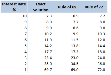
$$ln \left( 1 + \frac{i}{100} \right) = \frac{r}{100} – \frac{r^2}{20000} + … $$
In our case, it is more convenient to write this as:
$$ln \left( 1 + \frac{i}{100} \right) = \frac{1}{100} \left( r – \frac{r^2}{200} + … \right) $$
For $r<10$, the second term is less than $\frac{100}{200} = 0.5$. Given the first term is of the order $10$, this means we are only throwing out an adjustment of less than $5 \%$ to our final answer.

Taking just the first term of the Taylor expansion, we end up with:
$$n \approx \frac{69.3 \%}{\frac{1}{100} * \frac{1}{r}}$$
And rearranging gives:
$$n \approx \frac{69.3}{r}$$
So we see, we are pretty close to $ n \approx \frac{72}{r}$.
​
Why 72?

We saw above that using just the first term of the Taylor Expansion suggests we should be using the ‘rule of 69.3%' instead. Why then is this the rule of 72?
​
There are two main reasons, the first is that for most of the interest rates we are interested in, the Rule of 72 actually gives a better approximation to the exact solution, the following table compares the exact solution, the approximation given by the ‘Rule of 69’, and the approximation given by the Rule of 72:

The reason for this is that for interest rates in the 4%-10% range, the second term of the Taylor expansion is not completely negligible, and act to make the denominator slightly smaller and hence the fraction slightly bigger. It turns out 72 is quite a good fudge factor to account for this.
​
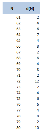
Another reason for using 72 over other close numbers is that 72 has a lot of divisors, in particular out of all the integers within 10 of 72, 72 has the most divisors. The following table displays the divisors function d(n), for values of n between 60 and 80. 72 clearly stands out as a good candidate.

​The rule of 72 in Actuarial Modelling

The main use I find for this trick is in mentally adjusting historic claims for claims inflation. I know that if I put in 6% claims inflation, my trended losses will double in size from their original level approximately every 12 years. Other uses include when analysing investment returns, thinking about the effects of monetary inflation, or it can even be useful when thinking about the effects of discounting.
​
Can we apply the Rule of 72 anywhere else?

As an aside, we should be careful when attempting to apply the rule of 72 over too long a time period. Say we are watching a movie set in 1940, can we use the Rule of 72 to estimate what values in the movie are equivalent to now? Let's set up an example and see why it doesn't really work in practice. Let's suppose an item in our movie costs 10 dollars.  First we need to pick an average inflation rate for the intervening period (something in the range of 3-4% is probably reasonable). We can then reason as follows; 1940 was 80 years ago, at 4% inflation, $\frac{72}{4} = 18$, and we’ve had approx. 4 lots of 18 years in that time. Therefore the price would have doubled 4 times, or will now be a factor of 16. Suggesting that 10 dollars in 1940 is now worth around 160 dollars in today's terms.

It turns out that this doesn’t really work though, let’s check it against another calculation. The average price of a new car in 1940 was around 800 dollars and the average price now is around 35k, which is a factor of 43.75, quite a bit higher than 16. The issue with using inflation figures like these over very long time periods, is for a given year the difference in the underlying goods is fairly small, therefore a simple percentage change in price is an appropriate measure. When we chain together a large number of annual changes, after a certain number of years, the underlying goods have almost completely changed from the first year to the last. For this reason, simply multiplying an inflation rate across decades completely ignores both improvements in the quality of goods over time, and changes in standards of living, so doesn't really convey the information that we are actually interested in.
​

What is a floating deductible?

Excess of Loss contacts for Aviation books, specifically those covering airline risks (planes with more than 50 seats) often use a special type of deductible,  called a floating deductible. Instead of applying a fixed amount to the loss in order to calculate recoveries, the deductible varies based on the size of the market loss and the line written by the insurer. These types of deductibles are reasonably common, I’d estimate something like 25% of airline accounts I’ve seen have had one.

As an aside, these policy features are almost always referred to as deductibles, but technically are not actually deductibles from a legal perspective, they should probably be referred to as floating attachment instead. The definition of a deductible requires that it be deducted from the policy limit rather than specifying the point above which the policy limit sits. That’s a discussion for another day though!

The idea is that the floating deductible should be lower for an airline on which an insurer takes a smaller line, and should be higher for an airline for which the insurer takes a bigger line. In this sense they operate somewhat like a surplus lines contract in property reinsurance.

Before I get into my issues with them, let’s quickly review how they work in the first place.

An example

When binding an Excess of Loss contract with a floating deductible, we need to specify the following values upfront:

• Limit = USD18.5m
• Fixed attachment = USD1.5m
• Original Market Loss = USD150m

And we need to know the following  additional information about a given loss in order to calculate recoveries from said loss:

• The insurer takes a 0.75% line on the risk
• The insurer’s limit is USD 1bn
• The risk suffers a USD 200m market loss.

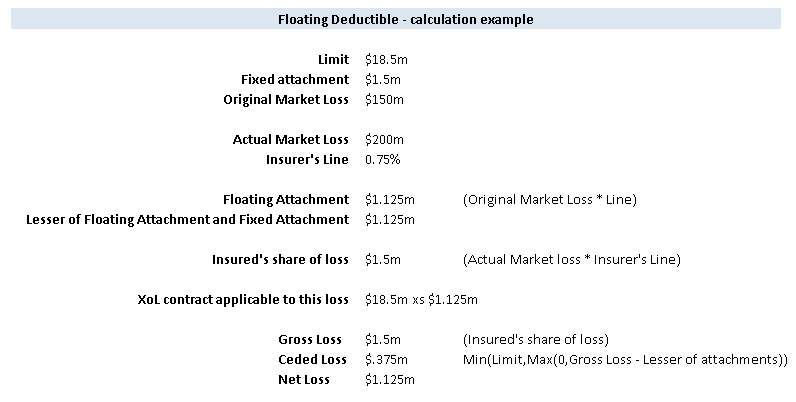
A standard XoL recovery calculation with the fixed attachment given above, would first calculate the UNL (200m*0.75%=1.5m), and then deduct the fixed attachment from this (1.5m-1.5m=0). Meaning in this case, for this loss and this line size, nothing would be recovered from the XoL.

To calculate the recovery from XoL with a floating deductible, we would once again calculate the insured’s UNL 1.5m. However we now need to calculate the applicable deductible, this will be the lesser of 1.5m (the fixed attachment), and the insurer’s effective line (defined as their UNL divided by the market loss = 1.5m/200m) multiplied by the Original Market Loss as defined in the contract. In this case, the effective line would be 0.75%, and the Original Market Loss would be 150m, hence; 0.75%*150m = 1.125m. Since this is less than the 1.5m fixed attachment, the attachment we should use is 1.125m our limit is always just 18.5m, and doesn’t change if the attachment drops down. We would therefore calculate recoveries to this contract, for this loss size and risk, as if the layer was a 18.5m xs 1.125. Meaning the ceded loss would be 0.375m, and the net position would be 1.125m.
​
Here’s the same calculation in an easier to follow format:

So…. what’s the issue?

This may seem quite sensible so far, however the issue is with the wording. The following is an example of a fairly standard London Market wording, taken from an anonymised slip which I came across a few years ago.

Priority: USD 10,000,000 each and every loss or an amount equal to the “Reinsured’s Portion’  of the total Original Insured Loss sustained by the original insured(s) of USD 200,000,000 each and every loss, whichever the lesser.
…
Reinsuring Clause
Reinsurers shall only be liable if and when the ultimate net loss paid by the Reinsured in respect of the interest as defined herein exceeds USD 10,000,000 each and every loss or an amount equal to the Reinsured’s Proportion of the total Original Insured Loss sustained by the original insured(s) of USD 200,000,000 or currency equivalent, each and every loss, whichever the lesser (herein referred to as the “Priority”)
For the purpose herein, the Reinsured’s Proportion shall be deemed to be a percentage calculated as follows, irrespective of the attachment dates of the policies giving rise to the Reinsured’s ultimate net loss and the Original Insured Loss:
Reinsured Ultimate Net Loss
/
Original Insured Loss
…
The Original Insured Loss shall be defined as the total amount incurred by the insurance industry including any proportional co-insurance and or self-insurance of the original insured(s), net of any recovery from any other source
What’s going on here is that we’ve defined the effective line to be the Reinsured’s unl divided by the 100% market loss.

First problem

From a legal perspective, how would an insurer (or reinsurer for that matter), prove what the 100% insured market loss is? The insurer obviously knows their share of the loss, however what if this is a split placement with 70% placed in London on the same slip, 15% placed in a local market (let’s say Indonesia?), and a shortfall cover (15%) placed in Bermuda. Due to the different jurisdictions, let’s say the Bermudian cover has a number of exclusions and subjectivities, and the Indonesian cover operates under the Indonesian legal system which does not publically disclose private contract details.

Even if the insurer is able to find out through a friendly broker what the other markets are paying, and therefore have a good sense of what the 100% market loss is, they may not have a legal right to this information. The airline does have a legal right to the information, however the reinsurance contract is a contract between the insured and reinsured, the airline is not a party to the reinsurance contract. The point is whether the insurer and reinsured have the legal right to the information.

The above issues may sound quite theoretical, and in practice there are normally no issues with collecting on these types of contracts. But to my mind, legal language should bear up to scrutiny even when stretched – that’s precisely when you are going to rely on it.  My contention is that as a general rule, it is a bad idea to rely on information in a contract which you do not have an automatic legal right to obtain.

The second problem

The intention with this wording, and with contracts of this form is that the effective line should basically be the same as the insured’s signed line. Assuming everything is straightforward, if the insurer takes a x% line with a limit of Y bn. If the loss is anything less than Y bn, then the insured’s effective line will simply be x%*Size of Loss / Size of loss. i.e. x%.

My guess as to why it is worded this way rather than just taking the actual signed line is that we don’t want to open ourselves to a issues around what exactly we mean by ‘the signed line’ – what if the insured has exposure through two contracts both of which have different signed lines, what if there is an inuring Risk Excess which effectively nets down the gross signed line – should we then use the gross or net line? By couching the contract in terms of UNLs and Market losses we attempt to avoid these ambiguities

Let me give you a scenario though where this wording does fall down:

Scenario 1 – clash loss

Let’s suppose there is a mid-air collision between two planes. Each results in an insured market loss of USD 1bn, then the Original Insured Loss is  USD 2bn. If our insurer takes a 10% line on the first airline, but does not write the second airline, then their effective line is 10% * 1bn / 2bn = 5%... hmmm this is definitely equal to their signed line of 10%.

You may think this is a pretty remote possibility, after all in the history of modern commercial aviation such an event has not occurred. What about the following scenario which does occur fairly regularly?

Scenario 2 – airline/manufacturer split liability

Suppose now there is a loss involving a single plane, and the size of the loss is once again USD 1bn, and that our insurer once again has a 10% line. In this case though, what if the manufacturer is found 50% responsible? Now the insurer only has a UNL of USD 500m, and yet once again, in the calculation of their floating deductible, we do the following:  10% * 500m/1bn = 5%.

Hmmm, once again our effective line is below our signed line, and the floating deductible will drop down even further than intended.

Suggested alternative wording

My suggested wording, and I’m not a lawyer so this is categorically not legal advice, is to retain the basic definition of effective line - as UNL divided by some version of the 100% market loss -  by doing so we still neatly sidestep the issues mentioned above around gross vs net lines, or exposure from multiple slips, but instead to replace the definition of Original Insured Loss with some variation of the following ‘the proportion of the Original Insured Loss, for which the insured derives a UNL through their involvement in some contract of insurance, or otherwise’.

Basically the intention is to restrict the market loss, only to those contracts through which the insurer has an involvement. This deals with both issues – the insurer would not be able to net down their line further through references to insured losses which are nothing to do with them, as in the case of scenario 1 and 2 above, and secondly it restrict the information requirements to contracts which the insurer has an automatic legal right to have knowledge of since by definition they will be a party to the contract.

I did run this idea past a few reinsurance brokers a couple of years ago, and they thought it made sense. The only downside from their perspective is that it makes the client's reinsurance slightly less responsive i.e. they knew about the strange quirk whereby the floating deductible dropped in the event of a manufacturer involvement, and saw it as a bonus for their client, which was often not fully priced in by the reinsurer. They therefore had little incentive to attempt to drive through such a change. The only people who would have an incentive to push through this change would be the larger reinsurers, though I suspect they will not do so until they've already been burnt and attempted to rely on the wording in a court case and, at which point they may find it does not quite operate in the way they intended.