|
On why it doesn’t really make sense to fit a Pareto distribution with a method of moments.
I was sent some large loss modelling recently by another actuary for a UK motor book. In the modelling, they had taken the historic large losses, and fit a Pareto distribution using a method of moments. I thought about it for a while and realized that it didn't really like the approach for a couple of reasons which I'll go into in more detail below, but then when I thought about it some more I realised I'd actually seen the exact approach before ... in an IFoA exam paper. So even though the method has some shortcomings, it is actually a taught technique. [1]

Following the theme from last time, of London's old vs new side by side. Here's a cool photo which shows the old royal naval college in Greenwich, with Canary Wharf in the background. Photo by Fas Khan
We've been playing around in the last few posts with the 'Nth largest' method of analysing claims inflation. I promised previously that I would look at the effect of increasing the volatility of our severity distribution when using the method, so that's what we are going to look at today. Interestingly it does have an effect, but it's actually quite a subdued one as we'll see.

I'm running out of ideas for photos relating to inflation, so here's a cool random photo of New York instead. Photo by Ronny Rondon
Capped or uncapped estimators9/6/2023 I was reviewing a pricing model recently when an interesting question came up relating to when to apply the policy features when modelling the contract.  Source: Dall.E 2, Open AI.
I thought it would be fun to include an AI generated image which was linked to the title 'capped vs uncapped estimators'. After scrolling through tons of fairly creepy images of weird looking robots with caps on, I found the following, which is definitely my favourite - it's basically an image of a computer 'wearing' a cap. A 'capped' estimator... The Lomax pareto distribution in SciPy17/3/2023 The Python library SciPy, contains a version of the Lomax distribution which it defines as: $$f(x,c) = \frac{c}{(a+x)^{(c+1)}}$$ Whereas, the ‘standard’ specification is [1]: $$f(x,c, \lambda) = \frac{c \lambda ^ c}{(a+x)^{(c+1)}}$$ Which is also the definition in the IFoA core reading [2]:  So, how can we use the SciPy version of the Lomax to simulate the standard version, given we are missing the $ \lambda ^c$ term?
MLE of a Uniform Distribution28/2/2023 I noticed something surprising about the Maximum Likelihood Estimator (MLE) for a uniform distribution yesterday. Suppose we’re given sample $X’ = {x_1, x_2, … x_n}$ from a uniform distribution $X$ with parameters $a,b$. Then the MLE estimator for $a = min(X’)$, and $b = max(X’)$. [1] All straight forward so far. However, examining the estimators, we can also say with probability = 1 that $a < min(X’)$, and similarly that $b > max(X’)$. Isn't it strange that the MLE estimators are clearly less/more than the true values? So what can we do instead?  (Since Gauss did a lot of the early work on MLE, here's a portrait of him as a young man. )
Source: https://commons.wikimedia.org/wiki/File:Bendixen_-_Carl_Friedrich_Gau%C3%9F,_1828.jpg The official Microsoft documentation for the Excel Forecast.ETS function is pretty weak [1]. Below I’ve written a few notes on how the function works, and the underlying formulas.  Source: Microsoft office in Seattle, @Coolcaesar, https://en.wikipedia.org/wiki/File:Building92microsoft.jpg
Aggregating probability forecasts18/3/2022 There's some interesting literature from the world of forecasting and natural sciences on the best way to aggregate predictions from multiple models/sources. For a well-written, moderately technical introduction, see the following by Jaime Sevilla: forum.effectivealtruism.org/posts/sMjcjnnpoAQCcedL2/when-pooling-forecasts-use-the-geometric-mean-of-odds Jaime’s article suggests a geometric mean of odds as the preferred method of aggregating predictions. I would argue however that when it comes to actuarial pricing, I'm more of a fan of the arithmetic mean, I'll explain why below.  Bayesian Analysis vs Actuarial Methods21/4/2021
David Mackay includes an interesting Bayesian exercise in one of his books [1]. It’s introduced as a situation where a Bayesian approach is much easier and more natural than equivalent frequentist methods. After mulling it over for a while, I thought it was interesting that Mackay only gives a passing reference to what I would consider the obvious ‘actuarial’ approach to this problem, which doesn’t really fit into either category – curve fitting via maximum likelihood estimation.
On reflection, I think the Bayesian method is still superior to the actuarial method, but it’s interesting that we can still get a decent answer out of the curve fitting approach. The book is available free online (link at the end of the post), so I’m just going to paste the full text of the question below rather than rehashing Mackay’s writing: I received an email from a reader recently asking the following (which for the sake of brevity and anonymity I’ve paraphrased quite liberally)
I’ve been reading about the Poisson Distribution recently and I understand that it is often used to model claims frequency, I’ve also read that the Poisson Distribution assumes that events occur independently. However, isn’t this a bit of a contradiction given the policyholders within a given risk profile are clearly dependent on each other? It’s a good question; our intrepid reader is definitely on to something here. Let’s talk through the issue and see if we can gain some clarity. Stirling's Approximation23/2/2020 I’m reading ‘Information Theory, inference and learning algorithms' by David MacKay at the moment and I'm really enjoying it so far. One cool trick that he introduces early in the book is a method of deriving Stirling’s approximation through the use of the Gaussian approximation to the Poisson Distribution, which I thought I'd write up here.
Constructing Probability Distributions9/11/2019
There is a way of thinking about probability distributions that I’ve always found interesting, and to be honest I don’t think I’ve ever seen anyone else write about it. For each probability distribution, the CDF can be thought of as a partial infinite sum, or partial integral identity, and the probability distribution is uniquely defined by this characterisation (with a few reasonable conditions)
I think at this point most people will either have no idea what I'm talking about (probably because I've explained it badly), or they’ll think what I’ve just said is completely obvious. Let me give an example to help illustrate. Poisson Distribution as a partial infinite sum Start with the following identity:
$$ \sum_{i=0}^{\infty} \frac{ x^i}{i!} = e^{x}$$
And let's bring the exponential over to the other side. $$ \sum_{i=0}^{\infty} \frac{ x^i}{i!} e^{-x} = 1$$ Let's state a few obvious facts about this equation; firstly, this is an infinite sum (which I claimed above were related to probability distributions - so good so far). Secondly, the identity is true by the definition of $e^x$, all we need to do to prove the identity is show the convergence of the infinite sum, i.e. that $e^x$ is well defined. Finally, each individual summand is greater than or equal to 0. With that established, if we define a function: $$ F(x;k) = \sum_{i=0}^{k} \frac{ x^i}{i!} e^{-x}$$ That is, a function which specifies as its parameter the number of partial sumummads we should add together. We can see from the above identity that:
But wait, the formula for $F(x;k)$ above is actually just the formula for the CDF of a Poisson random variable! That’s interesting right? We started with an identity involving an infinite sum, we then normalised it so that the sum was equal to 1, then we defined a new function equal to the partial summation from this normalised series, and voila, we ended up with the CDF of a well-known probability distribution. Can we repeat this again? (I’ll give you a hint, we can) Exponential Distribution as a partial infinite integral Let’s examine an integral this time. We’ll use the following identity: $$\int_{0}^{ \infty} e^{- \lambda x} dx = \lambda$$ An integral is basically just a type of infinite series, so let’s apply the same process, first we normalise: $$ \frac{1}{\lambda} \int_{0}^{ \infty} e^{- \lambda x} dx = 1$$ Then define a function equal to the partial integral: $$ F(y) = \frac{1}{\lambda} \int_{0}^{ y} e^{- \lambda x} dx $$ And we've ended up with the CDF of an Exponential distribution! Euler Integral of the first kind This construction even works when we use more complicated integrals. The Euler integral of the first kind is defined as:
$$B(x,y)=\int_{0}^{1}t^{{x-1}}(1-t)^{{y-1}} dt =\frac{\Gamma (x)\Gamma (y)}{\Gamma (x+y)}$$
This allows us to normalise:
$$\frac{\int_{0}^{1}t^{{x-1}}(1-t)^{{y-1}}dt}{B(x,y)} = 1$$ And once again, we can construct a probability distribution: $$B(x;a,b) = \frac{\int_{0}^{x}t^{{a-1}}(1-t)^{{b-1}}dt}{B(a,b)}$$ Which is of course the definition of a Beta Distribution, this definition bears some similarity to the definition of an exponential distribution in that our normalisation constant is actually defined by the very integral which we are applying it to. Conclusion So can we do anything useful with this information? Well not particularly. but I found it quite insightful in terms of how these crazy formulas were discovered in the first place, and we could potentially use the above process to derive our own distributions – all we need is an interesting integral or infinite sum and by normalising and taking a partial sum/integral we've defined a new way of partitioning the unit interval. Hopefully you found that interesting, let me know if you have any thoughts by leaving a comment in the comment box below! Beta Distribution in Actuarial Modelling3/11/2019
I saw a useful way of parameterising the Beta Distribution a few weeks ago that I thought I'd write about.
The standard way to define the Beta is using the following pdf:
$$f(x) = \frac{x^{\alpha -1} {(1-x)}^{\beta -1}}{B ( \alpha, \beta )}$$
Where $ x \in [0,1]$ and $B( \alpha, \beta ) $ is the Beta Function:
$$ B( \alpha, \beta) = \frac{ \Gamma (\alpha ) \Gamma (\beta)}{\Gamma(\alpha + \beta)}$$
When we use this parameterisation, the first two moments are:
$$E [X] = \frac{ \alpha}{\alpha + \beta}$$
$$Var (X) = \frac{ \alpha \beta}{(\alpha + \beta)^2(\alpha + \beta + 1)}$$
We see that the mean and the variance of the Beta Distribution depend on both parameters - $\alpha$ and $\beta$. If we want to fit these parameters to a data set using a method of moments then we need to use the following formulas, which are quite complicated:
$$\hat{\alpha} = m \Bigg( \frac{m (1-m) }{v} - 1 \Bigg) $$
$$\hat{\beta} = (1- m) \Bigg( \frac{m (1-m) }{v} - 1 \Bigg) $$ This is not the only possible parameterisation of the Beta Distribution however. We can use an alternative definition where we define:
$$\gamma = \frac{ \alpha}{\alpha + \beta} $$, and $$\delta = \alpha + \beta$$
And then by construction, $E[X] = \gamma$, and we can calculate the new variance:
$$V = \frac{ \alpha \beta}{(\alpha + \beta)^2(\alpha + \beta + 1)} = \frac{\gamma ( 1 - \gamma)}{(1-\delta)}$$.
Placing these new variables back in our pdf gives the following equation:
$$f(x) = \frac{x^{\gamma \delta -1} {(1-x)}^{\delta (1-\gamma) -1}}{B ( \gamma \delta, \delta (1-\gamma) -1 )}$$
So why would we bother to do this? Our new formula now looks more complicated to work with than the one we started with. There are however two main advantages to this new version, firstly the method of moments is much simpler to set up, our first parameter is simply the mean, and the formula for variance is easier to calculate than before. This makes using the Beta distribution much easier in a Spreadsheet. The second advantage, and in my mind the more important point, is that since we now have a strong link between the central moments and the two parameters that define the distribution we now have an easy and intuitive understand of what our parameters actually represent. As I’ve written about before, rather than just sticking with the standard statistics textbook version, I’m a big fan of pushing parameterisations that are both useful and easily interpretable, The version of the Beta Distribution presented above achieves this. Furthermore it also fits nicely with the schema I've written about before (most recently in the in the post below on negative binomial distribution), in which no matter which distribution we are talking about, the first parameter of a distribution gives you information about it's mean, the second parameter gives information about its volatility, etc. By doing this you give yourself the ability to compare distributions and sense check parameterisations at a glance. Negative Binomial in VBA21/9/2019
Have you ever tried to simulate a negative binomial random variable in a Spreadsheet?
If the answer to that is ‘nope – I’d just use Igloo/Metarisk/Remetrica’ then consider yourself lucky! Unfortunately not every actuary has access to a decent software package, and for those muddling through in Excel, this is not a particularly easy task. If on the other hand your answer is ‘nope – I’d use Python/R, welcome to the 21st century’. I’d say great, I like using those programs as well, but sometimes for reasons out of your control, things just have to be done in Excel. This is the situation I found myself in recently, and here is my attempt to solve it: Attempt 0 The first step I took in attempting to solve the problem was of course to Google it, then cross my fingers and hope that someone else has already solved it and this is just going to be a simple copy and paste. Unfortunately when I did search for VBA code to generate a negative binomial random variable, nothing comes up. In fact, nothing comes up when searching for code to simulate a Poisson random variable in VBA. Hopefully if you've found your way here, looking for this exact thing, then you're in luck, just scroll to the bottom and copy and paste my code. When I Googled it, there were a few solutions that almost solved the problem; there is a really useful Excel add-in called ‘Real statistics’ which I’ve used a few times: http://www.real-statistics.com/ It's a free excel add-in, and it does have functionality to simulate negative bimonials. If however you need someone to be able to re-run the Spreadsheet, they also will need to have it installed. In that case, you might as well use Python, and then hard code the frequency numbers. Also, I have had issues with it slowing Excel down considerably, so I decided not to use this in this case. I realised I’d have to come up with something myself, which ideally would meet the following criteria
How hard can that be? Attempt 1 I’d seen a trick before (from Pietro Parodi’s excellent book ‘Pricing in General Insurance’) that a negative binomial can be thought of as a Poisson distribution with a Gamma distribution as the conjugate prior. See the link below for more details: https://en.wikipedia.org/wiki/Conjugate_prior#Table_of_conjugate_distributions Since Excel has a built in Gamma inverse, we have simplified the problem to needing to write our own Poisson inverse. We can then easily generate negative binomials using a two step process:
Great, so we’ve reduced our problem to just being able to simulate a Poisson in VBA. Unfortunately there’s still no built in Poisson inverse in Excel (or at least the version I have), so we now need a VBA based method to generate this. There is another trick we can use for this - which is also taken from Pietro Parodi - the waiting time for a Poisson dist is an Exponential Dist. And the CDF of an Exponential dist is simple enough that we can just invert it and come up with a formula for generating an Exponential sample. We then set up a loop and add together exponential values, to arrive at Poisson sample. The code for this is give below:
Function Poisson_Inv(Lambda As Double)

    s = 0
    N = 0
    Do While s < 1
        u = Rnd()
        s = s - (Application.WorksheetFunction.Ln(u) / Lambda)
        k = k + 1
    Loop
    Poisson_Inv = (k - 1)

End Function
The VBA code for our negative binomial is therefore:
Function NegBinOld2(b, r)

    Dim Lambda As Double
    Dim N As Long

    u = Rnd()

    Lambda = Application.WorksheetFunction.Gamma_Inv(u, r, b)

    N = Poisson_Inv(Lambda)

    NegBinOld2 = N

End Function
Does this do everything we want?
There are a couple of downside of though:
This leads us on to Attempt 2 Attempt 2 If we pass the VBA a random uniform sample, then whenever we hit refresh in the Spreadsheet the random sample will refresh, which will force the Negative Binomial to resample. Without this, sometimes the VBA will function will not reload. i.e. we can use the sample to force a refresh whenever we like. Adapting the code gives the following:
Function NegBinOld(b, r, Rnd1 As Double)

    Dim Lambda As Double
    Dim N As Long

    u = Rnd1

    Lambda = Application.WorksheetFunction.Gamma_Inv(u, r, b)

    N = Poisson_Inv(Lambda)

    NegBinOld = N

End Function
So this solves the refresh problem. What about the random seed problem? Even though we now always get the same lambda for a given rand – and personally I quite like to hardcode these in the Spreadsheet once I’m happy with the model, just to speed things up. We still use the VBA rand function to generate the Poisson, this means everytime we refresh, even when passing it the same rand, we will get a different answer and this answer will be non-replicable. This suggests we should somehow use the first random uniform sample to generate all the others in a deterministic (but still pseudo-random) way. Attempt 3 The way I implemented this was to the set the seed in VBA to be equal to the uniform random we are passing the function, and then using the VBA random number generator (which works deterministically for a given seed) after that. This gives the following code:
Function NegBin(b, r, Rnd1 As Double)

    Rnd (-1)
    Randomize (Rnd1)

    Dim Lambda As Double
    Dim N As Long

    u = Rnd()

    Lambda = Application.WorksheetFunction.Gamma_Inv(u, r, b)

    N = Poisson_Inv(Lambda)

    NegBin = N

End Function
So we seem to have everything we want – a free, quick, solution that can be bundled in a Spreadsheet, which allows other people to rerun without installing any software, and we’ve also eliminated the forced refresh issue. What more could we want? The only slight issue with the last version of the negative binomial is that our parameters are still specified in terms of ‘b’ and ‘r’. Now what exactly are ‘b’ and ‘r’ and how do we relate them to our sample data? I’m not quite sure.... The next trick is shamelessly taken from a conversation I had with Guy Carp’s chief Actuary about their implementation of severity distributions in MetaRisk. Attempt 4 Why can't we reparameterise the distribution using parameters that we find useful, instead of feeling bound by using the standard statistics textbook definition (or even more specifically the list given in the appendix to ‘Loss Models – from data to decisions’, which seems to be somewhat of an industry standard), why can't we redefine all the parameters from all common actuarial distributions using a systematic approach for parameters? Let's imagine a framework where no matter which specific severity distribution you are looking at, the first parameter contains information about the mean (even better if it is literally scaled to the mean in some way), the second contains information about the shape or volatility, the third contains information about the tail weight, and so on. This makes fitting distributions easier, it makes comparing the goodness of fit of different distributions easier, and it make sense checking our fit much easier. I took this idea, and tied this in neatly to a method of moments parameterisation, whereby the first value is simply the mean of the distribution, and the second is the variance over the mean. This gives us our final version:
Function NegBin(Mean, VarOMean, Rnd1 As Double)

    Rnd (-1)
    Randomize (Rnd1)

    Dim Lambda As Double
    Dim N As Long

    b = VarOMean - 1
    r = Mean / b

    u = Rnd()

    Lambda = Application.WorksheetFunction.Gamma_Inv(u, r, b)

    N = Poisson_Inv(Lambda)

    NegBin = N

End Function

Function Poisson_Inv(Lambda As Double)

    s = 0
    N = 0
    Do While s < 1
        u = Rnd()
        s = s - (Application.WorksheetFunction.Ln(u) / Lambda)
        k = k + 1
    Loop
    Poisson_Inv = (k - 1)

End Function
Poisson Distribution for small Lambda23/4/2019
I was asked an interesting question a couple of weeks ago when talking through some modelling with a client.
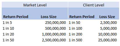
We were modelling an airline account, and for various reasons we had decided to base our large loss modelling on a very basic top-down allocation method. We would take a view of the market losses at a few different return periods, and then using a scenario approach, would allocate losses to our client proportionately. Using this method, the frequency of losses is then scaled down by the % of major policies written, and the severity of losses is scaled down by the average line size. To give some concrete numbers (which I’ve made up as I probably shouldn’t go into exactly what the client’s numbers were), let's say the company was planning on taking a line on around 10% of the Major Airline Risks, and their average line was around 1%. We came up with a table of return periods for market level losses. The table looked something like following (the actual one was also different to the table below, but not miles off): 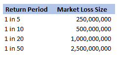
Then applying the 10% hit factor if there is a loss, and the 1% line written, we get the following table of return periods for our client:
Hopefully all quite straightforward so far. As an aside, it is quite interesting to sometimes pare back all the assumptions to come up with something transparent and simple like the above. For airline risks, the largest single policy limit is around USD 2.5bn, so we are saying our worst case scenario is a single full limit loss, and that each year this has around a 1 in 50 chance of occurring. We can then directly translate that into an expected loss, in this case it equates to 50m (i.e. 2.5bn *0.02) of pure loss cost. If we don't think the market is paying this level of premium for this type of risk, then we better have a good reason for why we are writing the policy!
So all of this is interesting (I hope), but what was the original question the client asked me? We can see from the chart that for the market level the highest return period we have listed is 1 in 50. Clearly this does translate to a much longer return period at the client level, but in the meeting where I was asked the original question, we were just talking about the market level. The client was interested in what the 1 in 200 at the market level was and what was driving this in the modelling. The way I had structured the model was to use four separate risk sources, each with a Poisson frequency (lambda set to be equal to the relevant return period), and a fixed severity. So what this question translates to is, for small Lambdas $(<<1)$, what is the probability that $n=2$, $n=3$, etc.? And at what return period is the $n=2$ driving the $1$ in $200$? Let’s start with the definition of the Poisson distribution: Let $N \sim Poi(\lambda)$, then: $$P(N=n) = e^{-\lambda} \frac{ \lambda ^ n}{ n !} $$ We are interested in small $\lambda$ – note that for large $\lambda$ we can use a different approach and apply sterling’s approximation instead. Which if you are interested, I’ve written about here: www.lewiswalsh.net/blog/poisson-distribution-what-is-the-probability-the-distribution-is-equal-to-the-mean
For small lambda, the insight is to use a Taylor expansion of the $e^{-\lambda}$ term. The Taylor expansion of $e^{-\lambda}$ is:
$$ e^{-\lambda} = \sum_{i=0}^{\infty} \frac{\lambda^i}{ i!} = 1 - \lambda + \frac{\lambda^2}{2} + o(\lambda^2) $$
We can then examine the pdf of the Poisson distribution using this approximation: $$P(N=1) =\lambda e^{-\lambda} = \lambda ( 1 – \lambda + \frac{\lambda^2}{2} + o(\lambda^2) ) = \lambda - \lambda^2 +o(\lambda^2)$$
as in our example above, we have:
$$ P(N=1) ≈ \frac{1}{50} – {\frac{1}{50}}^2$$
This means that, for small lambda, the probability that $N$ is equal to $1$ is always slightly less than lambda. Now taking the case $N=2$: $$P(N=2) = \frac{\lambda^2}{2} e^{-\lambda} = \frac{\lambda^2}{2} (1 – \lambda +\frac{\lambda^2}{2} + o(\lambda^2)) = \frac{\lambda^2}{2} -\frac{\lambda^3}{2} +\frac{\lambda^4}{2} + o(\lambda^2) = \frac{\lambda^2}{2} + o(\lambda^2)$$
So once again, for $\lambda =\frac{ 1}{50}$ we have:
$$P(N=2) ≈ 1/50 ^ 2 /2 = P(N=1) * \lambda / 2$$
In this case, for our ‘1 in 50’ sized loss, we would expect to have two such losses in a year once every 5000 years! So this is definitely not driving our 1 in 200 result.
We can add some extra columns to our market level return periods as follows: 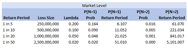
So we see for the assumptions we made, around the 1 in 200 level our losses are still primarily being driven by the P(N=1) of the 2.5bn loss, but then in addition we will have some losses coming through corresponding to P(N=2) and P(N=3) of the 250m and 500m level, and also combinations of the other return periods.
So is this the answer I gave to the client in the meeting? …. Kinda, I waffled on a bit about this kind of thing, but then it was only after getting back to the office that I thought about trying to breakdown analytically which loss levels we can expect to kick in at various return periods. Of course all of the above is nice but there is an easier way to see the answer, since we’d already stochastically generated a YLT based on these assumptions, we could have just looked at our YLT, sorted by loss size and then gone to the 99.5 percentile and see what sort of losses make up that level. The above analysis would have been more complicated if we have also varied the loss size stochastically. You would normally do this for all but the most basic analysis. The reason we didn’t in this case was so as to keep the model as simple and transparent as possible. If we had varied the loss size stochastically then the 1 in 200 would have been made up of frequency picks of various return periods, combined with severity picks of various return periods. We would have had to arbitrarily fix one in order to say anything interesting about the other one, which would not have been as interesting. Extending the Copula Method26/8/2018 If you have ever generated Random Variables stochastically using a Gaussian Copula, you may have noticed that the correlation of the generated sample ends up being lower than the value of the Covariance matrix of the underlying multivariate Gaussian Distribution. For an explanation of why this happens you can check out a previous post of mine: www.lewiswalsh.net/blog/correlations-friedrich-gauss-and-copula. It would be nice if we could amend our method to compensate for this drop. As a quick fix, we can simply run the model a few times and fudge the Covariance input until we get the desired Correlation value. If the model runs quickly, this is quite easy to do, but as soon as the model starts to get bigger and slower, it quickly becomes impractical to run it three of four times just to get the output Correlation we desire. We can do better than this. The insight we rely on is that for a Gaussian Copula, the Pearson Correlation in the generated sample just depends on the Covariance Value. We can therefore create a precomputed table of Input and Output values, and use this to select the correct input value for the desired output. I wrote some R code to do just that, we compute a table of Pearson's Correlations obtained for various Input Covariance values when using the Gaussian Copula.
a <- library(MASS)
library(psych)

set.seed(100)

m <- 2
n <- 10^6

OutputCor <- 0
InputCor <- 0

for (i in 1:100) {

  sigma <- matrix(c(1, i/100,
                    i/100, 1),
                  nrow=2)
  z <- mvrnorm(n,mu=rep(0, m),Sigma=sigma,empirical=T)

  u <- pnorm(z)

  OutputCor[i] <- cor(u,method='pearson')[1,2]
  InputCor[i] <- i/10

}

OutputCor
InputCor
Here is a sample from the table of results. You can see that the drop is relatively modest, but it does apply consistent across the whole table. 
Here is a graph showing the drop in values: 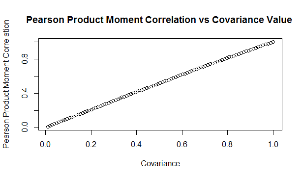
Updated Algorithm
We can then use the pre-computed table, interpolating where necessary, to give us a Covariance value for our Multivariate Gaussian Distribution which will generate the desired Pearson Product Moment Correlation Value. So for example, if we would like to generate a sample with a Pearson Product Moment value of $0.5$, according to our table, we would need to use $0.517602$ as an input Covariance. We can test these values using the following code:
a <- library(MASS)
library(psych)

set.seed(100)

m <- 2
n <- 5000000
sigma <- matrix(c(1, 0.517602,
                  0.517602, 1),
                nrow=2)
z <- mvrnorm(n,mu=rep(0, m),Sigma=sigma,empirical=T)
u <- pnorm(z)

cor(u,method='pearson')
Analytic Formulas I tried to find an analytic formula for the Product Moment values obtained in this manner, but I couldn't find anything online, and I also wasn't able to derive one myself. If we could find one, then instead of using the precompued table, we would be able to simply calculate the correct value. While searching, I did come across a number of interesting analytic formulas linking the values of Kendall's Tau, Spearman's Rank, and the input Covariance.. All the formulas below are from Fang, Fang, Kotz (2002) Link to paper: www.sciencedirect.com/science/article/pii/S0047259X01920172 The paper gives the following two results, where $\rho$ is the Pearson's Product Moment
$$\tau = \frac{2}{\pi} arcsin ( \rho ) $$ $$ {\rho}_s = \frac{6}{\pi} arcsin ( \frac{\rho}{2} ) $$
We can then use these formulas to extend our method above further to calculate an input Covariance to give any desired Kendall Tau, or Spearman's Rank. I initially thought that they would link the Pearson Product Moment value with Kendall or Spearman's measure, in which case we would still have to use the precomputed table. After testing it I realised that it is actually linking the Covariance to Kendall and Spearman's measures. Thinking about it, Kendall's Tau, and Spearman's Rank are both invariant to the reverse Gaussian transformation when moving from $z$ to $u$ in the algorithm. Therefore the problem of deriving an analytic formula for them is much simpler as one only has to link their values for a multivariate Gaussian Distribution. Pearson's however does change, therefore it is a completely different problem and may not even have a closed form solution. As an example of how to use the above formula, suppose we'd like our generated data to have a Kendall's Tau of $0.4$. First we need to invert the Kendall's Tau formula: $$ \rho = sin ( \frac{ \tau \pi }{2} ) $$ We then plug in $\rho = 0.4 $ giving:
$$ \rho = sin ( \frac{ o.4 \pi }{2} ) = 0.587785 $$
Giving usan input Covariance value of $0.587785$
We can then test this value with the following R code:
a <- library(MASS)
library(psych)

set.seed(100)

m <- 2
n <- 50000
sigma <- matrix(c(1, 0.587785,
                  0.587785, 1),
                nrow=2)
z <- mvrnorm(n,mu=rep(0, m),Sigma=sigma,empirical=T)
u <- pnorm(z)
cor(z,method='kendall')
Which we see gives us the value of $\tau$ we want. In this case the difference between the input Covariance $0.587785$, and the value of Kendall's Tau $0.4$ is actually quite significant. |
AuthorI work as an actuary and underwriter at a global reinsurer in London. Categories
All
Archives
April 2024
|
 RSS Feed