​Every year we have an office sweepstake for the Cheltenham horse racing festival. Like most sweepstakes, this one attempts to remove the skill, allowing everyone to take part without necessarily needing to know much about horse racing.

In case you’re not familiar with a Sweepstake, here’s a simple example of how one based on the World Cup might work:

• Entry costs £5
• Each player randomly selects a team
• The player who picked the team that goes on to win, gets all the money

This allows anyone to enter and have an equal chance of winning (the chance is equal prior to drawing, but not equal once the draw has been made), otherwise everyone would just want Spain or Germany, or whichever team is currently considered the favourite.
 
Note that in order for this to work properly, you need to ensure that the team draw is not carried out until everyone who wants to play has put their money in – otherwise you introduce some optionality and people can then decide whether to enter based on the teams that are still left. i.e. if you know that Germany and Spain have already been picked then there is less value in entering the competition.
 
The rules for our Cheltenham sweepstake were as follows:
 
The Rules
 
The festival comprises 7 races a day for 4 days, for a total of 28 races.
 
The sweepstake costs £20 to enter, and the winnings are calculated as follows:
 
3rd place in competition = 10% of pot
2nd place in competition = 20% of pot
1st place in competition = 70% of pot
 
Each participant picks one horse per race each morning. Points are then calculated using the following scoring system:

• 1st place – 5 x odds
• 2nd place – 3 x odds
• 3rd place – 1 x odds

 
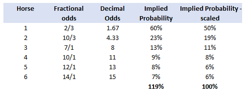
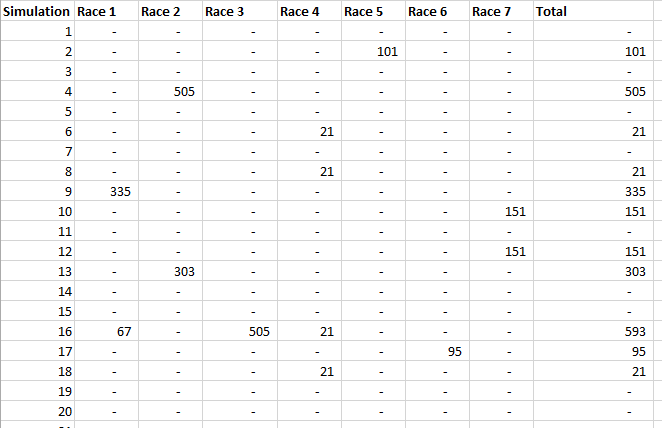
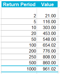
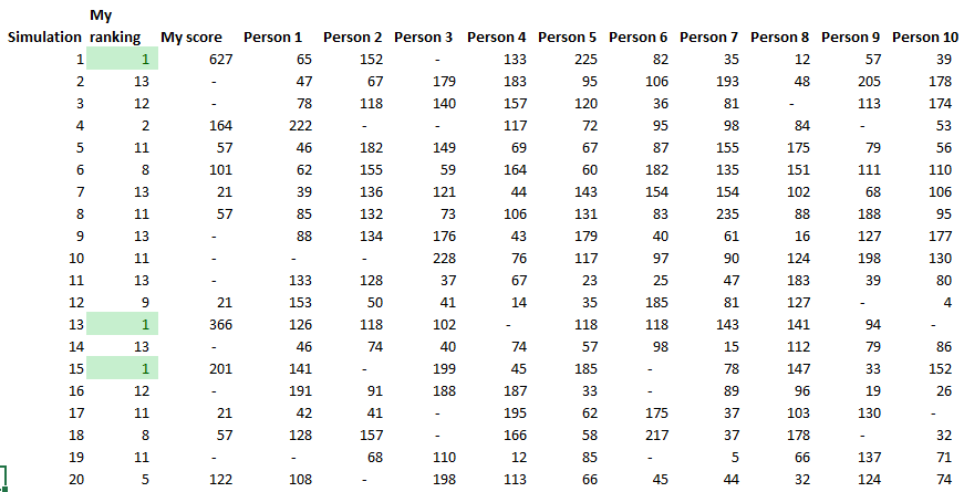
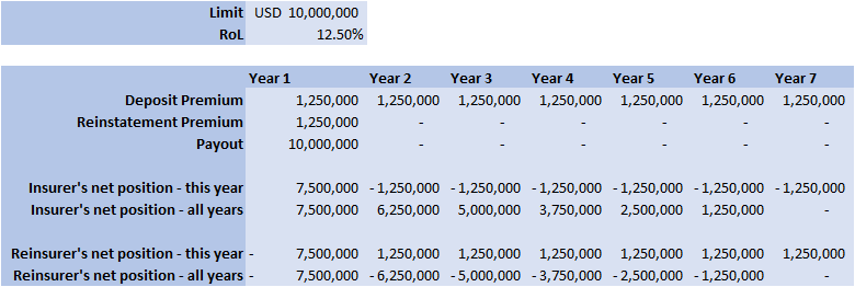
A running total is kept throughout the competition, and the winner is determined after the final race.
 
The odds the scoring are based on are set using the odds printed in the Metro Newspaper on the morning of the races.
 
(as an example, for a horse which has odds of 11/2 in the Metro - if the horse then places 1st, if we selected this horse, we would win (1+11/2)*5 = 32.5 points)
 
Initial thoughts
 
Any set of betting odds can be converted to an implied probability of winning, these would be the odds which over the long run would cause you to breakeven if the race were repeated multiple times with each horse winning a proportion equal to its probability of winning.

Because the scoring in our sweepstake is based on the betting odds, using implied probabilities derived from the odds to help select our horses ends up cancelling itself out (which was the intention when designing the rules). The implied probability can be calculated as one over the odds As an aside, the bookie is indifferent to whether this is the correct probability of winning, they structures the odds purely on the ratio of how their customers are betting. They then structure the odds so that they make money on each race, regardless of which horse wins, for an explanation of this, see my post on creating a Dutchbook:
​
​www.lewiswalsh.net/blog/archives/12-2017
 
Here is an example showing how we would calculate the implied probabilities using some made up odds:
 

​

We can then use the implied probabilities we just calculated to see what would happen if each horse finished in the first three positions. Once we have done this, we can then calculate the Expected Value of betting on each horse:

We see that the payout varies for each horse, but the EV is the same. This is by design, the intention is that it should not matter which horse you bet on, the sweepstake rules equalise everyone.

So what can we - an actuary who knows nothing much about horse racing - do? I don’t have any special knowledge that would allow me to select a horse which would beat the odds listed in the Metro, we appear to be at an impasse.

I could attempt to build a model of which horse will win, and then select my horse based on that, but unless it proves to be more accurate than the Metro odds, I might as well just pick at random. Furthermore, if I could build such a model, then I could just start betting actual money. This probably shows you what a difficult problem this is! There's no such thing as free money. It would be a cool project to try, and it’s something I’ve been meaning to attempt for a while, but that’s best saved for another day.

Attempt 1 - Metro vs pre-race odds

My first thought was that we can exploit the difference in odds between those published in the Metro in the morning, and the latest odds published closer to the start of the race. It seems reasonable to assume that the odds just before the race should be more accurate than the metro odds. There will have been time for additional information to be included in the more up to date odds, e.g. the weather is worse than expected therefore horse x is expected to be slower than usual. Since the payout will be based on the Metro, we will then be able to maximise our EV by exploiting this differential. 

Our table will end up looking something like this:
​

 
We see that we have very small variations in the EVs for some of the horses. It looks like according to this analysis Horse 3 would be the best selection as it has the highest EVs for 1st, 2nd, and 3rd. Based on this strategy, we would then go through each race and select the horse with the highest EV.

Is this what I did? No, for a couple of reasons. The biggest issue was that the Metro did not publish odds in the morning for all races, meaning we couldn’t use the Metro, and therefore the rules of the sweepstake were amended to use the official pre-race odds to calculate the payout instead. This meant there was only one set of odds used, and our edge disappeared!
​
Even if we had used this method, there was a more fundamental issue - the margins we ended up with were tiny anyway. The Metro vs pre-race odds did not swing wildly, meaning that even selecting the horse with the highest EV were only marginally better than picking at random.

So, was there an alternative?

Attempt 2 - 2nd and 3rd place odds
​
My next attempt at an exploitative strategy was based on the insight that the payout multiplier for 2nd and 3rd place was based on the odds of the horse coming 1st, rather than the odds of the horse coming 2nd or 3rd.

The expected value of a horse was not quite as I calculated above, it was actually:
$$EV = P(1)*p_1 + P(2)*p_2 + P(3)*p_3$$
Above, we were using the implied probability of the horse coming first as a proxy for the probability it would come second and third. This is not the same, and some betting websites do allow you to bet on whether a horse will come 2nd or 3rd.

For websites that do not allow you to bet directly on this, then we may still be able to calculate it from the odds for whether a horse finishes in the top 2 or 3 places. We just need to subtract out the implied probability of coming 1st from the probability of coming in the top 2, and then subtracting this out from coming top 3 etc.

​I therefore added some more columns to my table above, corresponding to the probability of the horses coming 2nd and 3rd, and then used this to calculate the EV instead.

We see that the final column, Total EV, now has quite different values for each horse. In this case Horse 15, Seddon has an EV of 11.72. The favourite horse on the other hand - number 7  - only has an EV of 6.2. The intuitive explanation of this is that the probability of Seddon coming first is very low – this is the reflected in the long odds of 67, this then gives us a large multiplier, but the odds of the horse coming second or third are actually relatively less far out – the fact that it is not the favourite actually increases the odds of it coming in a position which is not 1st. But then if does come in 2nd or 3rd, we would still apply the same large multiplier for the odds of it coming 1st. This then gives us our 2nd edge – we can gain a positive EV by focusing.

As a thought experiment, imagine we have a race with three horses – horse A is a clear favourite, horse B is an average horse, and horse C is clearly the weakest. By betting on horse C – the odds of it winning should be very low, so the multiple should be very high, but then this multiple will be applied even if it comes 2nd or 3rd, which is exactly where it is expected to finish.

This therefore suggests our next potential strategy – select horses which maximise our EV using the implied probabilities of the horses coming 2nd, 3rd etc.

So is this what I did? Well kind of....

The issue with this approach is that typically the horses that provide the best EV also have very long odds. In the race analysed above, our horse has an EV of 11.7, but it only has a 7% chance overall of coming in the top 3. In race two for example, the horse with the best EV actually only had a 2.7% chance of coming in the top 3. Since there are only 28 races in total, if each horse we selected only had a 2.7% chance of coming in, then the probability of us getting 0 points overall in the entire competition would then be:
​
$(1-2.7 \%)^{28} = 48 \%$​

So there is roughly a 50% chance we will get 0 points!

Alternatively, if we selected the favourite every time, we could expect it to come top 3 almost every time, and thereby guarantee ourselves points most races, but it also has the lowest EV.

So we have what appears to be a risk vs reward trade off. Pick outsiders and give ourselves the highest EV overall, or pick the favourites thereby reducing our overall EV but also reducing our volatility.

This leads us  neatly to attempt 3 - trying to think about how to maximise our probability of winning the competition rather than simply maximising EV for each race.
​
Attempt 3 - EP curves
​
From the work above, we now have our model of the position each horse will finish in each race – using the 1st, 2nd, and 3rd implied probabilities - and we have the payout for each horse – using the odds of the horse coming 1st. We can then bring our selection of horse and these probabilities together in a summary tab and simulate our daily score stochastically using a Monte Carlo method. To do this we just need to turn the implied probabilities into a CDF, and lookup the value of each position and repeat 10,000 times. The output for this then ends up looking like the following, where the value is the number of points we will for a given race.

So we see that across this sample of 20 simulations, most days we to end up with 0 points overall, but a few days have very high scores. So far so good!

The next step is to set up an EP table of the following, which looks like the following:

The EP table gives us the probability of exceeding various scores in the competition based on our horse selections. In this case, we see that there is a 1 in 20 chance of getting 453 points or greater in the day.

This is useful even on its own – when I was deciding which horses to bet on, I simply played around with the selections until I got an EP table I was comfortable with. My reasoning was quite basic – I decided I wanted to maximise the 1 in 20 value. I wanted to give myself something like a 1/4 chance of winning the whole competition and a 3/4 chance of getting very few points. Since there were four days of races, dividing the 1/4 by another 4 suggests we should be looking at maximising the 1 in 20 level (I admit this reasoning was a bit rough, but it seemed to serve its purpose)

The insight here is that the payout structure of the sweepstake is such that coming in the top 3 is all that matters, and in particular coming 1st is disproportionately rewarded. To see this, we can think of the daily selection of horses as attempting to maximise the EV of the overall prize rather than the EV of our overall score - maximising the EV of each race is only a means to this end. So we are actually interested in maximising the following:

$0.7 * P(1st) + 0.2 + P(2nd) + 0.1 * P(3rd)$

Which will largely be dominated by P(1st), given the $0.7$ factor.
​
This is largely the strategy I went for in the end.

Attempt 4 - Game theory?

I’ve brushed over one difficulty above; in order to maximise our prize EV we need to consider not just which strategy we should take, but how this strategy will fare against the strategies that other people will take. If everyone is maximising their 1 in 20 return period then there’s little point us doing exactly the same. Luckily for me, most people were doing little more than picking horses randomly. We could then formalise this assumption, and come up with a numerical solution to the problem above.

To do this, we would simulate our returns for each day across 10,000 simulations as above, but this time we would compare ourselves against a ‘base strategy’ of random selection of horses and we would simulate this base strategy for the approximately 40 people who entered.

Each simulation would then give us a ranking we would finish in the competition, Here is an example of what that would look like:

​And we could then convert this into an EP table which would look like the following:

So we see that if we select these horses, we end up having somewhere between a 1 in 10 and a 1 in 5 chance of winning the competition.

Now that we have all of this set up, we can then optimise our horse selection to target a particular return period.

I didn’t actually end up setting up the above for the sweepstake, but I suspect it would have been an improvement on my approach

Attempt 5 - Multiple day?

There is a further refinement we can make to the above. We have so far only really been focusing on maximising our chance of winning by using a fixed strategy throughout the competition. But there is no reason we have to do this. After the first day, we should really be including the current scores of each competitor as part of our calculation of our ranking. i.e. if person 1 had a great day and now has 200 points but we had a bad day and still have 0 points, by accounting for this, the model should automatically increase our volatility i.e. start picking horses with longer odds so as to increase the chance of us catching up. If on the other hand, we had a really good first day and are now in the lead, the model should then automatically reduce our volatility and start selecting the favourites more often to help safely maintain our lead.
​
How did it work in practice?

I ended up placing 2nd, and taking 20% of the prize pot which was great! I was behind for most of the competition but then pulled back on the last day when a 66/1 came in 1st place, and I picked up 330 points off a single race. This may look miraculous, but is exactly how the model is supposed to work. 

Does that have any applicability to gambling generally? Unfortunately not, basically all of the work above is based on exploiting the specific scoring system of the sweepstake. There's no real way of apply this to gambling generally.

I came across a useful way of looking at Rate on Lines last week, I was talking to a broker about what return periods to use in a model for various levels of airline market loss (USD250m, USD500m, etc.). The model was intended to be just a very high level, transparent market level model which we could use as a framework to discuss with an underwriter. We were talking through the reasonableness of the assumptions when the broker came out with the following:
 
'Well, you’d pay about 12.5 on line in the retro market at that attachment level, so that’s a 1 in 7 break-even right?'
 
My response was:

'ummmm, come again?'
 
His reasoning was as follows:
 
Suppose the ILW pays $1$ @ $100$% reinstatements, and that it costs $12.5$​% on line.
Then if the layer suffers a loss, the insured will have a net position on the contract of $75$%. This is the $100$% limit which they receive due to the loss, minus the original $12.5$% Premium, minus an additional $12.5$% reinstatement Premium. The reinsurer will now need another $6$ years at $12.5$% RoL $(0.0125 * 6 = 0.75)$ to recover the limit and be at break-even.
 
Here is a breakdown of the cashflow over the seven years for a $10m$ stretch at $12.5$% RoL:
 

So the loss year plus the six clean years, tells us that if a loss occurs once every 7 years, then the contract is at break-even for this level of RoL.

So this is kind of cool - any time we have a RoL for a retro layer, we can immediately convert it to a Return Period for a loss which would trigger the layer.
 
Generalisation 1 – various rates on line
 
We can then generalise this reasoning to apply to a layer with an arbitrary RoL. Using the same reasoning as above, the break-even return period ends up being:
 
$RP= 1 + \frac{(1-2*RoL)}{RoL}$
 
Inverting this gives:
 
$RoL = \frac{1}{(1 + RP)}$
 
So let's say we have an ILW costing $7.5$% on line, the break-even return period is:
 
$1 + \frac{(1-0.15)}{0.075} = 11.3$
 
Or let’s suppose we have a $1$ in $19$ return period, the RoL will be:
 
$0.05 = \frac{1}{(1 + 19)}$
 
Generalisation 2 – other non-proportional layers
 
The formula we derived above was originally intended to apply to ILWs, but it also holds any time we think the loss to the layer, if it occurs, will be a total loss. This might be the case for a cat layer, or a clash layers (layers which have an attachment above the underwriting limit for a single risk), or any layer with a relatively high attachment point compared to the underwriting limit.
 
Adjustments to the formulas
 
There are a few of adjustments we might need to make to these formulas before using them in practice.
 
Firstly, the RoL above has no allowance for profit or expense loading, we can account for this by converting the market RoL to a technical RoL, this is done by simply dividing the RoL by $120-130$% (or any other appropriate profit/expense loading). This has the effect of increasing the number of years before the loss is expected to occur.
 
Alternately, if layer does not have a paid reinstatement, or has a different factor than $100$%, then we would need to amend the multiple we are multiplying the RoL by in the formula above. For example, with nil paid reinstatements, the formula would be:
 
$RP = 1 + \frac{(1-RoL)}{RoL}$
 
Another refinement we might wish to make would be to weaken the total loss assumption.  We would then need to reduce the RoL by an appropriate amount to account for the possibility of partial losses. It’s going to be quite hard to say how much this should be adjusted for – the lower the layer the more it would need to be.