Correlations, Friedrich Gauss, and Copulas

It's the second week of your new job Capital Modelling job. After days spent sorting IT issues, getting lost coming back from the toilets, and perfecting your new commute to work (probability of getting a seat + probability of delay * average journey temperature.) your boss has finally given you your first real project to work on.

You've been asked to carry out an annual update of the Underwriting Risk Capital Charge for a minor part of the company's Motor book. Not the grandest of analysis you'll admit, this particular class only makes up about 0.2% of the company's Gross Written Premium, and the Actuaries who reserve the company's bigger classes would probably consider the number of decimal places used in the annual report more material than your entire analysis. But you know in your heart of hearts that this is just another stepping stone on your inevitable meteoric rise to Chief Actuary in the Merger and Acquisition department, where one day you will pass judgement on billion dollar deals in-between expensive lunches with CFOs, and drinks with journalists on glamorous rooftop bars.

The company uses in-house reserving software, but since you're not that familiar with it, and because you want to make a good impression, you decide to carry out extensive checking of the results in Excel. You fire up the Capital Modelling Software (which may or may not have a name that means a house made out of ice), put in your headphones and grind it out.

Hours later you emerge triumphant, and you've really nailed it, your choice of correlation (0.4), and correlation method (Gaussian Copula) is perfect. As planned you run extracts of all the outputs, and go about checking them in Excel. But what's this? You set the correlation to be 0.4 in the software, but when you check the correlation yourself in Excel, it's only coming out at 0.384?! What's going on?

Simulating using Copulas

The above is basically what happened to me (minus most of the actual details. but I did set up some modelling with correlated random variables and then checked it myself in Excel and was surprised to find that the actual correlation in the generated output was always lower than the input.) I looked online but couldn't find anything explaining this phenomenon, so I did some investigating myself.

So just to restate the problem, when using Monte Carlo simulation, and generating correlated random variables using the Copula method. When we actually check the correlation of the generated sample, it always has a lower correlation than the correlation we specified when setting up the modelling.

My first thought for why this was happening was that were we not running enough simulations and that the correlations would eventually converge if we just jacked up the number of simulations. This is the kind of behaviour you see when using Monte Carlo simulation and not getting the mean or standard deviation expected from the sample. If you just churn through more simulations, your output will eventually converge. When creating Copulas using the Gaussian Method, this is not the case though, and we can test this.

I generated the graph below in R to show the actual correlation we get when generating correlated random variables using the Copula method for a range of different numbers of simulations. There does seem to be some sort of loose limiting behaviour, as the number of simulations increases, but the limit appears to be around 0.384 rather than 0.4.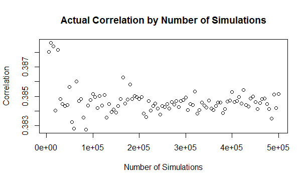

The actual explanation

First, we need to briefly review the algorithm for generating random variables with a given correlation using the normal copula.

Step 1 - Simulate from a multivariate normal distribution with the given covariance matrix.

Step 2 - Apply an inverse gaussian transformation to generate random variables with marginal uniform distribution, but which still maintain a dependency structure

Step 3 - Apply the marginal distributions we want to the random variables generated in step 2

We can work through these three steps ourselves, and check at each step what the correlation is.

The first step is to generate a sample from the multivariate normal. I'll use a correlation of 0.4 though out this example. Here is the R code to generate the sample:

a <- library(MASS)
library(psych)

set.seed(100)

m <- 2
n <- 1000
sigma <- matrix(c(1, 0.4,
                  0.4, 1), 
                nrow=2)
z <- mvrnorm(n,mu=rep(0, m),Sigma=sigma,empirical=T)

​

And here is a Scatterplot of the generated sample from the multivariate normal distribution: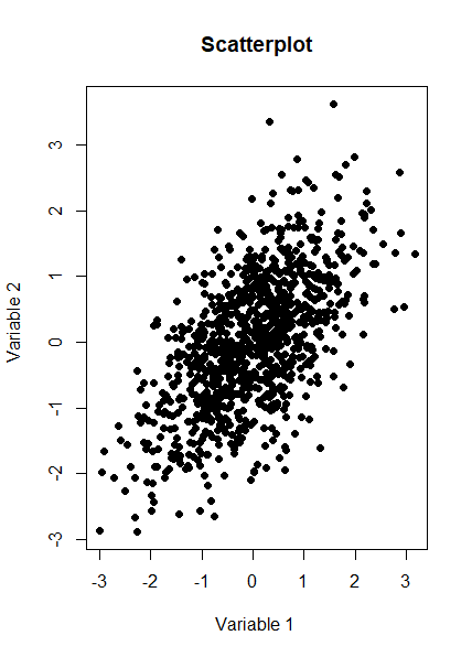
​

We now want to check the product moment correlation of our sample, which we can do using the following code:
​

cor(z,method='pearson')

Which gives us the following result:

> cor(z,method='pearson')
     [,1] [,2]
[1,]  1.0  0.4
[2,]  0.4  1.0

So we see that the correlation is 0.4 as expected. The Psych package has a useful function which produces a summary showing a Scatterplot, the two marginal distribution, and the correlation: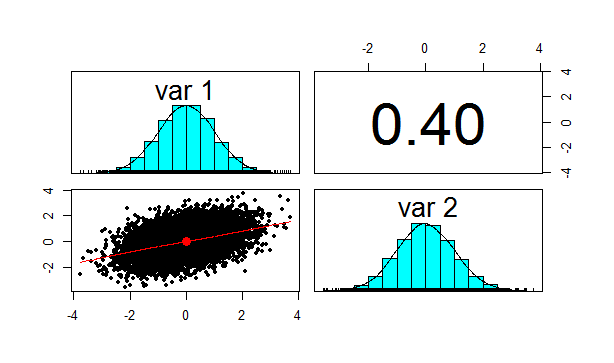

Let us also check Kendall's Tau and Spearman's rank at this point. This will be instructive later on. We can do this using the following code:

cor(z,method='spearman')

cor(z,method='Kendall')

Which gives us the following results:

> cor(z,method='spearman')
          [,1]      [,2]
[1,] 1.0000000 0.3787886
[2,] 0.3787886 1.0000000

> cor(z,method='kendall')
          [,1]      [,2]
[1,] 1.0000000 0.2588952
[2,] 0.2588952 1.0000000

Note that this is less than 0.4 as well, but we will discuss this further later on.

We now need to apply step 2 of the algorithm, which is applying the inverse Gaussian transformation to our multivariate normal distribution. We can do this using the following code:

u <- pnorm(z)

We now want to check the correlation again, which we can do using the following code:

cor(z,method='spearman')

Which gives the following result:

> cor(z,method='spearman')
          [,1]      [,2]
[1,] 1.0000000 0.3787886
[2,] 0.3787886 1.0000000

​Here is the Psych summary again: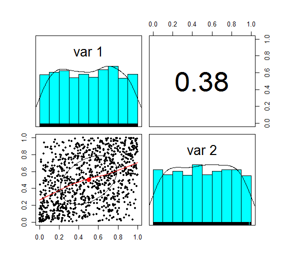

u is now marginally uniform (hence the name). We can see this by looking at the Scatterplot and marginal pdfs above.

We also see that the correlation has dropped to 0.379, down from 0.4 at step 1. The Pearson correlation measures the linear correlation between two random variables. We generated normal random variables, which had the required correlation, but then we applied a non-linear (inverse Gaussian) transformation. This non-linear step is the source of the dropped correlation in our algorithm.

We can also retest Kendall's Tau, and Spearman's at this point using the following code:

cor(z,method='spearman')

cor(z,method='Kendall')

This gives us the following result:

> cor(u,method='spearman')
          [,1]      [,2]
[1,] 1.0000000 0.3781471
[2,] 0.3781471 1.0000000

> cor(u,method='kendall')
          [,1]      [,2]
[1,] 1.0000000 0.2587187
[2,] 0.2587187 1.0000000

Interestingly, these values have not changed from above! i.e. we have preserved these measures of correlation between step 1 and step 2. It's only the Pearson correlation measure (which is a measure of linear correlation) which has not been preserved.

Let's now apply the step 3, and once again retest our three correlations. The code to carry out step 3 is below:

x1 <- qgamma(u[,1],shape=2,scale=1)
x2 <- qbeta(u[,2],2,2)

df <- cbind(x1,x2)
pairs.panels(df)

The summary for step 3 looks like the following.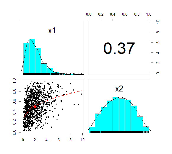

This is the end goal of our method. We see that our two marginal distributions have the required distribution, and we have a correlation between them of 0.37. Let's recheck our three measures of correlation.
​

cor(df,method='pearson')

cor(df,meth='spearman')

cor(df,method='kendall')

> cor(df,method='pearson')
          x1        x2
x1 1.0000000 0.3666192
x2 0.3666192 1.0000000

> cor(df,meth='spearman')
          x1        x2
x1 1.0000000 0.3781471
x2 0.3781471 1.0000000

> cor(df,method='kendall')
          x1        x2
x1 1.0000000 0.2587187
x2 0.2587187 1.0000000

So the Pearson has reduced again at this step, but the Spearman and Kendall's Tau are once again the same.

Does this matter?

This does matter, let's suppose you are carrying out capital modelling and using this method to correlate your risk sources. Then you would be underestimating the correlation between random variables, and therefore potentially underestimating the risk you are modelling.

Is this just because we are using a Gaussian Copula? No, this is the case for all Copulas. Is there anything you can do about it? Yes, one solution is to just increase the input correlation by a small amount, until we get the output we want.

A more elegant solution would be to build this scaling into the method. The amount of correlation lost at the second step is dependent just on the input value selected, so we could pre-compute a table of input and output correlations, and then based on the desired output, we would be able to look up the exact input value to use.