|
It's the second week of your new job Capital Modelling job. After days spent sorting IT issues, getting lost coming back from the toilets, and perfecting your new commute to work (probability of getting a seat + probability of delay * average journey temperature.) your boss has finally given you your first real project to work on. You've been asked to carry out an annual update of the Underwriting Risk Capital Charge for a minor part of the company's Motor book. Not the grandest of analysis you'll admit, this particular class only makes up about 0.2% of the company's Gross Written Premium, and the Actuaries who reserve the company's bigger classes would probably consider the number of decimal places used in the annual report more material than your entire analysis. But you know in your heart of hearts that this is just another stepping stone on your inevitable meteoric rise to Chief Actuary in the Merger and Acquisition department, where one day you will pass judgement on billion dollar deals in-between expensive lunches with CFOs, and drinks with journalists on glamorous rooftop bars. The company uses in-house reserving software, but since you're not that familiar with it, and because you want to make a good impression, you decide to carry out extensive checking of the results in Excel. You fire up the Capital Modelling Software (which may or may not have a name that means a house made out of ice), put in your headphones and grind it out. Hours later you emerge triumphant, and you've really nailed it, your choice of correlation (0.4), and correlation method (Gaussian Copula) is perfect. As planned you run extracts of all the outputs, and go about checking them in Excel. But what's this? You set the correlation to be 0.4 in the software, but when you check the correlation yourself in Excel, it's only coming out at 0.384?! What's going on? Simulating using Copulas The above is basically what happened to me (minus most of the actual details. but I did set up some modelling with correlated random variables and then checked it myself in Excel and was surprised to find that the actual correlation in the generated output was always lower than the input.) I looked online but couldn't find anything explaining this phenomenon, so I did some investigating myself. So just to restate the problem, when using Monte Carlo simulation, and generating correlated random variables using the Copula method. When we actually check the correlation of the generated sample, it always has a lower correlation than the correlation we specified when setting up the modelling. My first thought for why this was happening was that were we not running enough simulations and that the correlations would eventually converge if we just jacked up the number of simulations. This is the kind of behaviour you see when using Monte Carlo simulation and not getting the mean or standard deviation expected from the sample. If you just churn through more simulations, your output will eventually converge. When creating Copulas using the Gaussian Method, this is not the case though, and we can test this. I generated the graph below in R to show the actual correlation we get when generating correlated random variables using the Copula method for a range of different numbers of simulations. There does seem to be some sort of loose limiting behaviour, as the number of simulations increases, but the limit appears to be around 0.384 rather than 0.4. 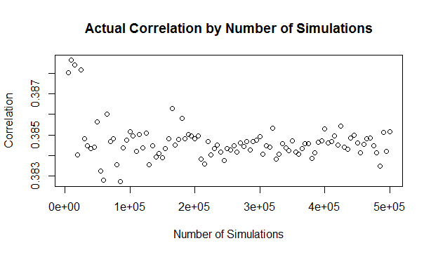
The actual explanation First, we need to briefly review the algorithm for generating random variables with a given correlation using the normal copula. Step 1 - Simulate from a multivariate normal distribution with the given covariance matrix. Step 2 - Apply an inverse gaussian transformation to generate random variables with marginal uniform distribution, but which still maintain a dependency structure Step 3 - Apply the marginal distributions we want to the random variables generated in step 2 We can work through these three steps ourselves, and check at each step what the correlation is. The first step is to generate a sample from the multivariate normal. I'll use a correlation of 0.4 though out this example. Here is the R code to generate the sample:
a <- library(MASS)
library(psych)
set.seed(100)
m <- 2
n <- 1000
sigma <- matrix(c(1, 0.4,
0.4, 1),
nrow=2)
z <- mvrnorm(n,mu=rep(0, m),Sigma=sigma,empirical=T)
And here is a Scatterplot of the generated sample from the multivariate normal distribution: 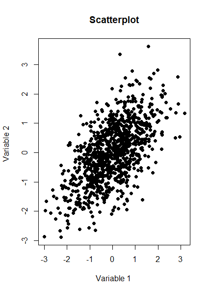
We now want to check the product moment correlation of our sample, which we can do using the following code: cor(z,method='pearson') Which gives us the following result: > cor(z,method='pearson') [,1] [,2] [1,] 1.0 0.4 [2,] 0.4 1.0 So we see that the correlation is 0.4 as expected. The Psych package has a useful function which produces a summary showing a Scatterplot, the two marginal distribution, and the correlation: 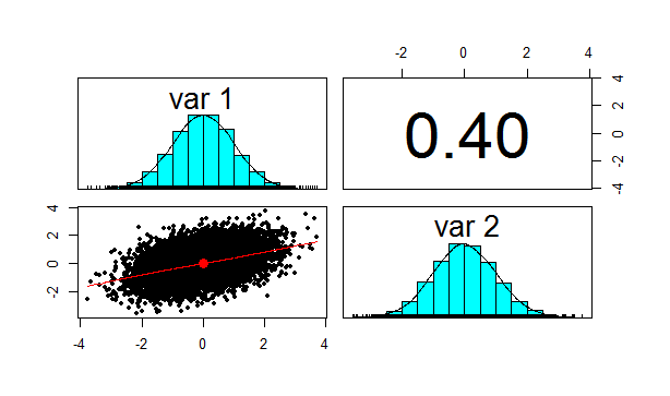
Let us also check Kendall's Tau and Spearman's rank at this point. This will be instructive later on. We can do this using the following code: cor(z,method='spearman') cor(z,method='Kendall') Which gives us the following results: > cor(z,method='spearman') [,1] [,2] [1,] 1.0000000 0.3787886 [2,] 0.3787886 1.0000000 > cor(z,method='kendall') [,1] [,2] [1,] 1.0000000 0.2588952 [2,] 0.2588952 1.0000000 Note that this is less than 0.4 as well, but we will discuss this further later on.
We now need to apply step 2 of the algorithm, which is applying the inverse Gaussian transformation to our multivariate normal distribution. We can do this using the following code:
u <- pnorm(z) We now want to check the correlation again, which we can do using the following code: cor(z,method='spearman') Which gives the following result: > cor(z,method='spearman') [,1] [,2] [1,] 1.0000000 0.3787886 [2,] 0.3787886 1.0000000 Here is the Psych summary again: 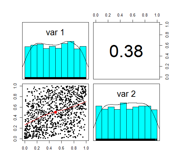
u is now marginally uniform (hence the name). We can see this by looking at the Scatterplot and marginal pdfs above. We also see that the correlation has dropped to 0.379, down from 0.4 at step 1. The Pearson correlation measures the linear correlation between two random variables. We generated normal random variables, which had the required correlation, but then we applied a non-linear (inverse Gaussian) transformation. This non-linear step is the source of the dropped correlation in our algorithm. We can also retest Kendall's Tau, and Spearman's at this point using the following code: cor(z,method='spearman') cor(z,method='Kendall') This gives us the following result: > cor(u,method='spearman') [,1] [,2] [1,] 1.0000000 0.3781471 [2,] 0.3781471 1.0000000 > cor(u,method='kendall') [,1] [,2] [1,] 1.0000000 0.2587187 [2,] 0.2587187 1.0000000 Interestingly, these values have not changed from above! i.e. we have preserved these measures of correlation between step 1 and step 2. It's only the Pearson correlation measure (which is a measure of linear correlation) which has not been preserved. Let's now apply the step 3, and once again retest our three correlations. The code to carry out step 3 is below: x1 <- qgamma(u[,1],shape=2,scale=1) x2 <- qbeta(u[,2],2,2) df <- cbind(x1,x2) pairs.panels(df) The summary for step 3 looks like the following. 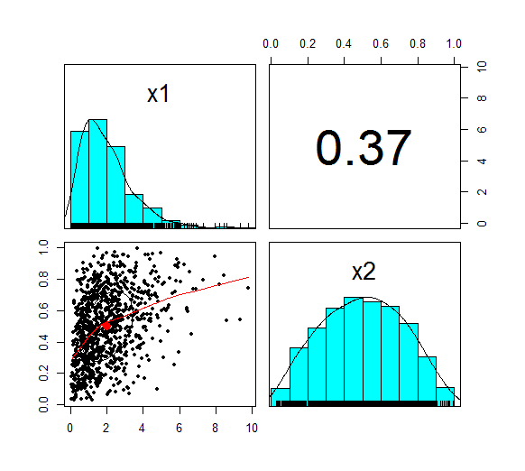
This is the end goal of our method. We see that our two marginal distributions have the required distribution, and we have a correlation between them of 0.37. Let's recheck our three measures of correlation. cor(df,method='pearson') cor(df,meth='spearman') cor(df,method='kendall') > cor(df,method='pearson') x1 x2 x1 1.0000000 0.3666192 x2 0.3666192 1.0000000 > cor(df,meth='spearman') x1 x2 x1 1.0000000 0.3781471 x2 0.3781471 1.0000000 > cor(df,method='kendall') x1 x2 x1 1.0000000 0.2587187 x2 0.2587187 1.0000000 So the Pearson has reduced again at this step, but the Spearman and Kendall's Tau are once again the same.
Does this matter?
This does matter, let's suppose you are carrying out capital modelling and using this method to correlate your risk sources. Then you would be underestimating the correlation between random variables, and therefore potentially underestimating the risk you are modelling. Is this just because we are using a Gaussian Copula? No, this is the case for all Copulas. Is there anything you can do about it? Yes, one solution is to just increase the input correlation by a small amount, until we get the output we want. A more elegant solution would be to build this scaling into the method. The amount of correlation lost at the second step is dependent just on the input value selected, so we could pre-compute a table of input and output correlations, and then based on the desired output, we would be able to look up the exact input value to use. If you have played around with Correlating Random Variables using a Correlation Matrix in [insert your favourite financial modelling software] then you may have noticed the requirement that the Correlation Matrix be positive semi-definite. But what exactly does this mean? And how would we check this ourselves in VBA or R? Mathematical Definition Let's start with the Mathematical definition. To be honest, it didn't really help me much in understanding what's going on, but it's still useful to know.
A symmetric $n$ x $n$ matrix $M$ is said to be positive semidefinite if the scalar $z^T M z $ is positive for every non-zero column vector $z$ of $n$ real numbers.
If I am remembering my first year Linear Algebra course correctly, then Matrices can be thought of as transformations on Vector Spaces. Here the Vector Space would be a collection of Random Variables. I'm sure there's some clever way in which this gives us some kind of non-degenerate behaviour. After a bit of research online I couldn't really find much. Intuitive Definition The intuitive explanation is much easier to understand. The requirement comes down to the need for internal consistency between the correlations of the Random Variables. For example, suppose we have three Random Variables, A, B, C. Let's suppose that A and B are highly correlated, that is to say, when A is a high value, B is also likely to be a high value. Let's also suppose that A and C are highly correlated, so that if A is a high value, then C is also likely to be a high value. We have now implicitly defined a constraint on the correlation between B and C. If A is high both B and C are also high, so it can't be the case that B and C are negatively correlated, i.e. that when B is high, C is low. Therefore some correlation matrices will give relations which are impossible to model. Alternative characterisations You can find a number of necessary and sufficient conditions for a matrix to be positive definite, I've included some of them below. I used number 2 in the VBA code for a real model I set up to check for positive definiteness. 1. All Eigenvalues are positive. If you have studied some Linear Algebra, then you may not be surprised to learn that there is a characterization using Eigenvalues. It seems like just about anything to do with Matrices can be restated in terms of Eigenvalues. I'm not really sure how to interpret this condition though in an intuitive way. 2. All leading principal minors are all positive This is the method I used to code the VBA algorithm below. The principal minors are just another name for the determinant of the upper-left $k$ by $k$ sub-matrix. Since VBA has a built in method for returning the determinant of a matrix this was quite an easy method to code. 3. It has a unique Cholesky decomposition I don't really understand this one properly, however I remember reading that Cholesky decomposition is used in the Copula Method when sampling Random Variables, therefore I suspect that this characterisation may be important! Since I couldn't really write much about Cholesky decomposition here is a picture of Cholesky instead, looking quite dapper. 
All 2x2 matrices are positive semi-definite Since we are dealing with Correlation Matrices, rather than arbitrary Matrices, we can actually show a-priori that all 2 x 2 Matrices are positive semi-definite. Proof
Let M be a $2$ x $2$ correlation matrix.
$$M = \begin{bmatrix} 1&a\\ a&1 \end{bmatrix}$$ And let $z$ be the column vector $M = \begin{bmatrix} z_1\\ z_2 \end{bmatrix}$ Then we can calculate $z^T M z$ $$z^T M z = {\begin{bmatrix} z_1\\ z_2 \end{bmatrix}}^T \begin{bmatrix} 1&a\\ a&1 \end{bmatrix} \begin{bmatrix} z_1\\ z_2 \end{bmatrix} $$ Multiplying this out gives us: $$ = {\begin{bmatrix} z_1\\ z_2 \end{bmatrix}}^T \begin{bmatrix} z_1 & a z_2 \\ a z_1 & z_2 \end{bmatrix} = z_1 (z_1 + a z_2) + z_2 (a z_1 + z_2)$$ We can then simplify this to get: $$ = {z_1}^2 + a z_1 z_2 + a z_1 z_2 + {z_2}^2 = (z_1 + a z_2)^2 \geq 0$$ Which gives us the required result. This result is consistent with our intuitive explanation above, we need our Correlation Matrix to be positive semidefinite so that the correlations between any three random variables are internally consistent. Obviously, if we only have two random variables, then this is trivially true, so we can define any correlation between two random variables that we like. Not all 3x3 matrices are positive semi-definite The 3x3 case, is simple enough that we can derive explicit conditions. We do this using the second characterisation, that all principal minors must be greater than or equal to 0.
Demonstration
Let M be a $3$ x $3$ correlation matrix: $$M = \begin{bmatrix} 1&a&b\\ a&1&c \\ b&c&1 \end{bmatrix}$$ We first check the determinant of the $2$ x $2$ sub matrix. We need that: $ \begin{vmatrix} 1 & a \\ a & 1 \end{vmatrix} \geq 0 $ By definition: $ \begin{vmatrix} 1 & a \\ a & 1 \end{vmatrix} = 1 - a^2$ We have that $ | a | \leq 1 $, hence $ | a^2 | \leq 1 $, and therefore: $ | 1- a^2 | \geq 0 $ Therefore the determinant of the $2$ x $2$ principal sub-matrix is always positive. Now to check the full $3$ x $3$. We require: $ \begin{vmatrix} 1 & a & b \\ a & 1 & c \\ b & c & 1 \end{vmatrix} \geq 0 $ By definition: $ \begin{vmatrix} 1 & a & b \\ a & 1 & c \\ b & c & 1 \end{vmatrix} = 1 ( 1 - c^2) - a (a - bc) + b(ac - b) = 1 + 2abc - a^2 - b^2 - c^2 $ Therefore in order for a $3$ x $3$ matrix to be positive demi-definite we require: $a^2 + b^2 + c^2 - 2abc = 1 $ I created a 3d plot in R of this condition over the range [0,1]. 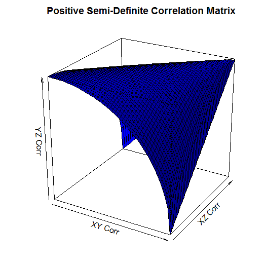
It's a little hard to see, but the way to read this graph is that the YZ Correlation can take any value below the surface. So for example, when the XY Corr is 1, and the XZ Corr is 0, the YZ Corr has to be 0. When the XY Corr is 0 on the other hand, and XZ Corr is also 0, then the YZ Corr can be any value between 0 and 1. Checking that a Matrix is positive semi-definite using VBA When I needed to code a check for positive-definiteness in VBA I couldn't find anything online, so I had to write my own code. It makes use of the excel determinant function, and the second characterization mentioned above. Note that we only need to start with the 3x3 sub matrix as we know from above that all 1x1 and all 2x2 determinants are positive. This is not a very efficient algorithm, but it works and it's quite easy to follow.
Function CheckCorrMatrixPositiveDefinite()
Dim vMatrixRange As Variant
Dim vSubMatrix As Variant
Dim iSubMatrixSize As Integer
Dim iRow As Integer
Dim iCol As Integer
Dim bIsPositiveDefinite As Boolean
bIsPositiveDefinite = True
vMatrixRange = Range(Range("StartCorr"), Range("StartCorr").Offset(inumberofrisksources - 1, inumberofrisksources - 1))
' Only need to check matrices greater than size 2 as determinant always greater than 0 when less than or equal to size 2'
If iNumberOfRiskSources > 2 Then
For iSubMatrixSize = iNumberOfRiskSources To 3 Step -1
ReDim vSubMatrix(iSubMatrixSize - 1, iSubMatrixSize - 1)
For iRow = 1 To iSubMatrixSize
For iCol = 1 To iSubMatrixSize
vSubMatrix(iRow - 1, iCol - 1) = vMatrixRange(iRow, iCol)
Next
Next
'If the determinant of the matrix is 0, then the matrix is semi-positive definite'
If Application.WorksheetFunction.MDeterm(vSubMatrix) < 0 Then
CheckCorrMatrixisPositiveDefinite = False
bIsPositiveDefinite = False
End If
Next
End If
If bIsPositiveDefinite = True Then
CheckCorrMatrixPositiveDefinite = True
Else
CheckCorrMatrixPositiveDefinite = False
End If
End Function
Checking that a Matrix is positive semi-definite in R Let's suppose that instead of VBA you were using an actually user friendly language like R. What does the code look like then to check that a matrix is positive semi-definite? All we need to do is install a package called 'Matrixcalc', and then we can use the following code: is.positive.definite( Matrix ) That's right, we needed to code up our own algorithm in VBA, whereas with R we can do the whole thing in one line using a built in function! It goes to show that the choice of language can massively effect how easy a task is.  I saw a cool trick the other day involving the Poisson Distribution and Stirling's Approximation. Given a Poisson Distribution $ N $ ~ $ Poi( \lambda ) $ The probability that $N$ is equal to a given $n$ is defined to be: $$P ( N = n) = \frac { {\lambda}^n e^{-n} } {n! } $$ What is the probability that $N$ is equal to it's mean? In this case, let's use $n$ as the mean of the distribution for reasons that will become clear later. Plugging $n$ into the definition of the Poisson distribution gives: $$P ( N = n) = \frac { n^n e^{-n} } {n! } $$ At this point, we use Sterling's approximation. Which states that for large $n$: $n!$ ~ $ {\left( \frac { n } {e } \right) }^n \frac { 1 } { \sqrt{ 2 \pi n } }$ Plugging this into the definition of the Poission Distribution gives: $$P ( N = n) = \frac { n^n e^{-n} } {{\left( \frac { n } {e } \right) }^n} \frac { 1 } { \sqrt{ 2 \pi n } } $$ Which simplifies to: $$P ( N = n) = \frac { 1 } { \sqrt{ 2 \pi n } } $$ So for large $n$ we end up with a nice result for the Probability that a Poisson Distribution will end up being equal to it's Expected Value. Convergence The convergence of the series is actually really quick. I checked the convergence for n between 1 and 50, and even by n=5, the approximation is very close, when I graphed it, the lines become indistinguishable very quickly. 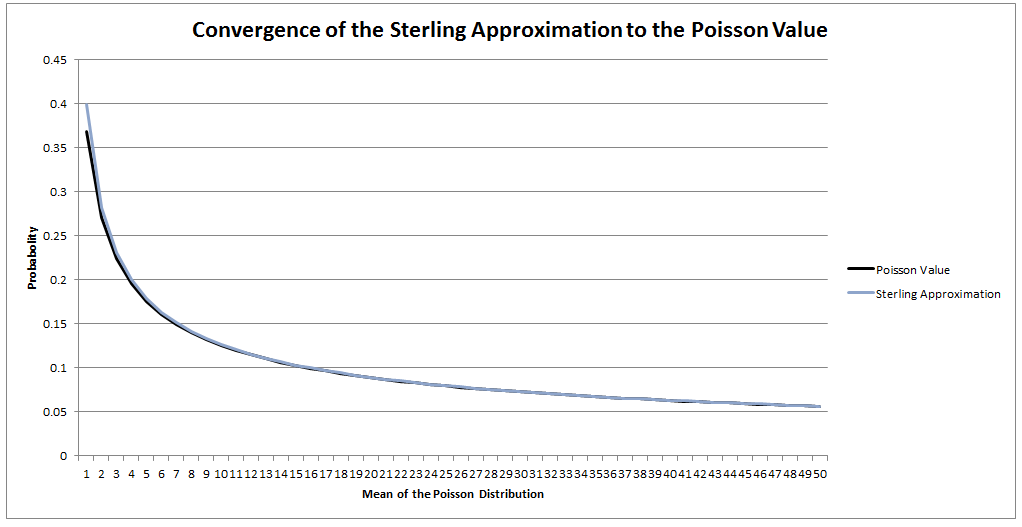 I could be on my own here, but personally I always thought the definition of Sample Standard Deviation is pretty ugly. $$ \sqrt {\frac{1}{n - 1} \sum_{i=1}^{n} { ( x_i - \bar{x} )}^2 } $$ We've got a square root involved which can be problematic, and what's up with the $\frac{1}{n-1}$? Especially the fact that it's inside the square root, also why do we even need a separate definition for a sample standard deviation rather than a population standard deviation? When I looked into why we do this, it turns out that the concept of sample standard deviation is actually a bit of a mess. Before we tear it apart too much though, let's start by looking at some of the properties of standard deviation which are good. Advantages of Standard Deviation
The last property is a really important one. The $\frac{1}{n-1}$ factor is a correction we make which we are told turns the sample standard deviation into an unbiased estimator of the population standard deviation. We can test this pretty easily, I sampled 50,000 simulations from a probability distribution and then measured the squared difference between the mean of the sample standard deviation and the actual value computed analytically. 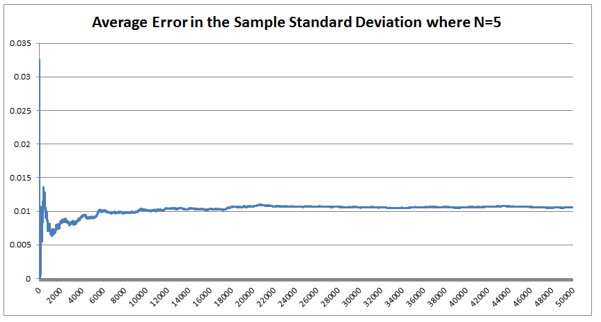 We see that the Average Error converges quite quickly but for some reason it doesn't converge to 0 as expected! It turns out that the usual formula for the sample standard deviation is not actually an unbiased estimator of the population standard deviation after all. I'm pretty sure they never mentioned that in my stats lectures at uni. The $n-1$ correction changes the formula for sample variance into an unbiased estimator, and the formula we use for the sample standard deviation is just the square root of the unbiased estimator for variance. If we do want an unbiased estimator for the sample standard deviation then we need to make an adjustment based not just on the sample size, but also the underlying distribution. Which in many cases we are not going to know at all. The wiki page has a good summary of the problem, and also has formulas for the unbiased estimator of the sample standard deviation: en.wikipedia.org/wiki/Unbiased_estimation_of_standard_deviation Just to give you a sense of the complexity, here is the factor that we need to apply to the usual definition of sample standard deviation in order to have an unbiased estimator for a normal distribution. $$ \frac {1} { \sqrt{ \frac{2}{n-1} } \frac{ \Gamma \Big( \frac{ n } {2} \Big) } {\Gamma \Big( \frac{n-1}{2} \Big)} } $$ Where $\Gamma$ is the Gamma function. Alternatives to Standard Deviation Are there any obvious alternatives to using standard deviation as our default measure of variability? Nassim Nicholas Taleb, author of Black Swan, is also not a fan of the wide spread use of the standard deviation of a distribution as a measure of its volatility. Taleb has different issues with it, mainly around the fact that it was often overused in banking by analysts who thought it completely characterised volatility. So for example, when modelling investment returns, an analyst would look at the sample standard deviation, and then assume the investment returns follow a Lognormal distribution with this standard deviation, when we should actually be modelling returns with a much fatter tailed distributions. So his issue was the fact that people believed that they were fully characterising volatility in this way, when they should have also been considering kurtosis and higher moments or considering fatter tailed distributions. Here is a link to Taleb's rant which is entertaining as always: www.edge.org/response-detail/25401 Taleb's suggestion is a different statistic called Mean Absolute Deviation the definition is. $$\frac{1}{n} \sum_{i=1}^n | x_i - \bar{x} | $$ We can see immediately why mathematicians prefer to deal with the standard deviation instead of the mean absolute deviation, working with sums of absolute values is normally much more difficult analytically than working with the square root of the sum of squares. In the ages of ubiquitous computing though, this should probably be a smaller consideration. |
AuthorI work as an actuary and underwriter at a global reinsurer in London. Categories
All
Archives
April 2024
|
 RSS Feed