|
We've been playing around in the last few posts with the 'Nth largest' method of analysing claims inflation. I promised previously that I would look at the effect of increasing the volatility of our severity distribution when using the method, so that's what we are going to look at today. Interestingly it does have an effect, but it's actually quite a subdued one as we'll see.

I'm running out of ideas for photos relating to inflation, so here's a cool random photo of New York instead. Photo by Ronny Rondon
So far when using the method, we've just left the mean and standard deviation of our severity distribution equal to 1m, and 1.5m respectively. When we did so, I made the observation that the standard deviation of our estimated inflation was around 1% with 20 years of data, and 0.5% with 30 years of data. These values are however dependent on the choice of severity standard deviation, so don't consider them to be some sort of universal constants. In order to understand the effect on the sampling error when varying the volatility of our losses, we're going to have to do some more modelling. In the code below, I loop through an array containing CVs ranging from 0.5 to 10 in 0.5 increments, which we will then be used to vary the severity distribution. We then record the standard deviation of our estimate using a (fixed) 20 years of data and provide the output as a graph.
In [1]:
import numpy as np
import pandas as pd
import scipy.stats as scipy
import matplotlib.pyplot as plt
from math import exp
from math import log
from math import sqrt
from scipy.stats import lognorm
from scipy.stats import poisson
from scipy.stats import linregress

import time
In [2]:
AverageFreq = 100
years = 20
ExposureGrowth = 0 #0.02

LLThreshold = 1e6
Inflation = 0.05

results=["Distmean","DistStdDev","AverageFreq","years","LLThreshold","Exposure Growth","Inflation"]

Distmean = 1500000.0

CV = [10,9.5,9,8.5,8,7.5,7,6.5,6,5.5,5,4.5,4,3.5,3,2.5,2,1.5,1,0.5]

AllMean = []
AllStdDev = []

for cv in CV:
    DistStdDev = Distmean*cv
    Mu = log(Distmean/(sqrt(1+DistStdDev**2/Distmean**2)))
    Sigma = sqrt(log(1+DistStdDev**2/Distmean**2))
    s = Sigma
    scale= exp(Mu)

    MedianTop10Method = []
    AllLnOutput = []

    for sim in range(5000):

        SimOutputFGU = []
        SimOutputLL = []
        year = 0
        Frequency= []
        for year in range(years):
            FrequencyInc = poisson.rvs(AverageFreq*(1+ExposureGrowth)**year,size = 1)
            Frequency.append(FrequencyInc)
            r = lognorm.rvs(s,scale = scale, size = FrequencyInc[0])
            r = np.multiply(r,(1+Inflation)**year)
            r_LLOnly = r[(r>= LLThreshold)]
            r_LLOnly = np.sort(r)[::-1]
            SimOutputLL.append(np.transpose(r_LLOnly))

        SimOutputLL = pd.DataFrame(SimOutputLL).transpose()
        a = np.log(SimOutputLL.iloc[5])
        AllLnOutput.append(a)
        b = linregress(a.index,a).slope
        MedianTop10Method.append(b)

    AllLnOutputdf = pd.DataFrame(AllLnOutput)

    dfMedianTop10Method= pd.DataFrame(MedianTop10Method)
    dfMedianTop10Method['Exp-1'] = np.exp(dfMedianTop10Method[0]) -1
    AllMean.append(np.mean(dfMedianTop10Method['Exp-1']))
    AllStdDev.append(np.std(dfMedianTop10Method['Exp-1']))

print(AllMean)
print(AllStdDev)

plt.plot(CV,AllStdDev)
plt.xlabel("Coefficient of Variation")
plt.ylabel("Standard deviation")
plt.show()
[0.05072302909044162, 0.05029059010555926, 0.05023576370167585, 0.05038584580882403, 0.05031722073338452, 0.049877493517084176, 0.04997320884626334, 0.05004169774475913, 0.050294936735433796, 0.05027466535297879, 0.04967237231808765, 0.05018616563017755, 0.0503642242825729, 0.04985468961621761, 0.049779840251667304, 0.04992333168150448, 0.0500177789651696, 0.0499908910094298, 0.05000765048199825, 0.05004972163569653] [0.018444672701967275, 0.01814411365805419, 0.017859624454479625, 0.01728234464859298, 0.017152730852483936, 0.017122682457061195, 0.016671245893483393, 0.01679034266455874, 0.016102135024973596, 0.015921409808456428, 0.015323929790813009, 0.015188295905687004, 0.014186494331466517, 0.013741673208871472, 0.012844921330655396, 0.012042476551892486, 0.010874335840823835, 0.009194050470380716, 0.00707976118467608, 0.004034548578398814] 
In [ ]:
Results Last time we ran the model, our CV was 1.5, and we had a standard deviation of 0.9%. Reading the value of CV = 1.5 off the above graph, we see that we are consistent with our previous modelling. Good start. We can see that as the CV increases, so do does the Std Dev of our inflation estimate, this is also in line with what we would expect. But luckily for us, the increase is fairly subdued. For example, we can increase our CV from 2 to 10, i.e. a 5 fold increase, and the Std Dev only increases by around a factor of 2. The best functional fit I could find for to the above graph was of the form a*sqrt(ln(x)), which worked reasonably well for CV >1.5. And just to note, if you remember your calculus 101, ln(x) is already a slowly increasing function, and we're adding on a sqrt operation which will make it even slower. So the increase is a very slow indeed. Here's the actual vs expected below: 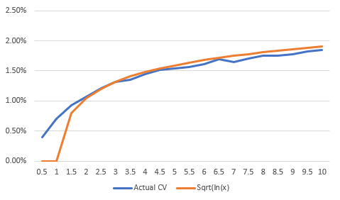
Conclusions If you recall from the previous post, we could reduce the standard deviation of the inflation estimate by including additional years of data $(N)$, at a rate of $b N^{(-c)}$ (with parameters around b = 0.45, c = 1.34, but which varied with the specific distribution). So we can always dominate the increase in the standard deviation of our estimate from additional volatility by including additional years of data. This is good! Had the functions been the other way around, then we would have reached a point where additional volatility in our underlaying severity distribution would have required exponentially more years of data in order to bring down. Not good! Next steps I still think there should be ways of getting more info out of our data, so next time lets maybe think about tweaking the method to see if it can be improved. |
AuthorI work as an actuary and underwriter at a global reinsurer in London. Categories
All
Archives
April 2024
|
 RSS Feed
Leave a Reply.