Bayesian Analysis vs Actuarial Methods

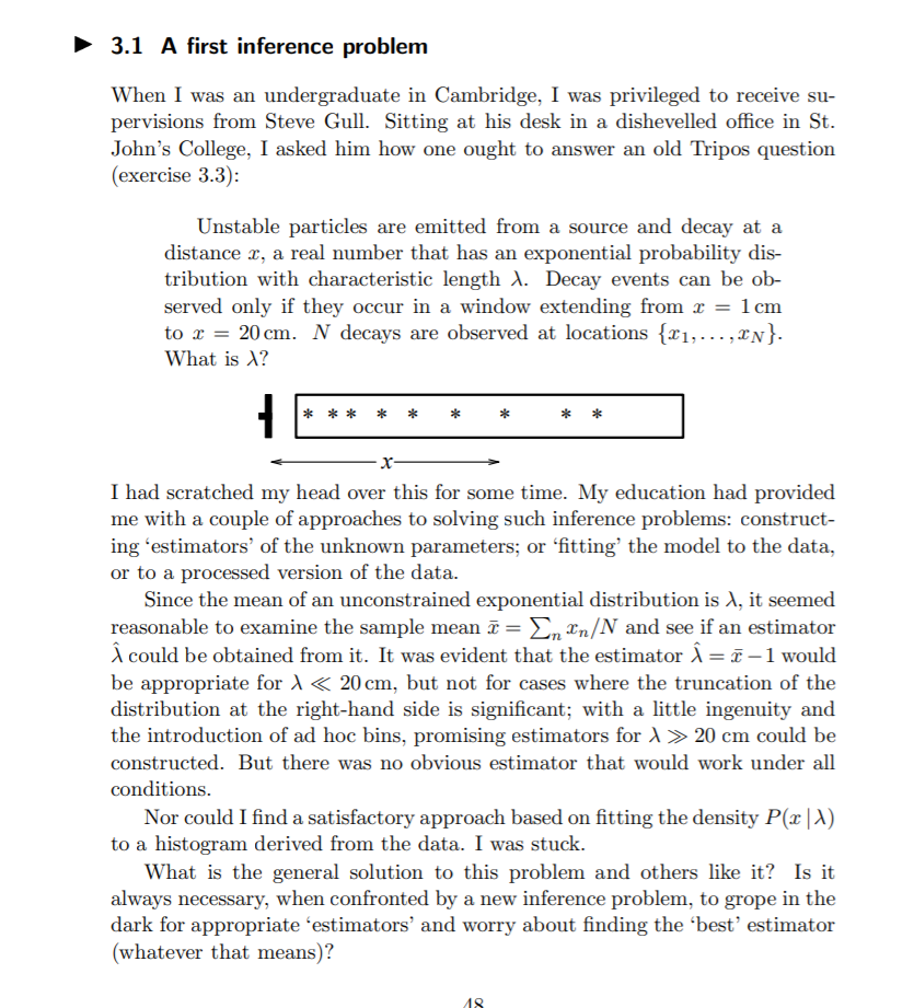
David Mackay includes an interesting Bayesian exercise in one of his books [1]. It’s introduced as a situation where a Bayesian approach is much easier and more natural than equivalent frequentist methods. After mulling it over for a while, I thought it was interesting that Mackay only gives a passing reference to what I would consider the obvious ‘actuarial’ approach to this problem, which doesn’t really fit into either category – curve fitting via maximum likelihood estimation.

On reflection, I think the Bayesian method is still superior to the actuarial method, but it’s interesting that we can still get a decent answer out of the curve fitting approach.

The book is available free online (link at the end of the post), so I’m just going to paste the full text of the question below rather than rehashing Mackay’s writing:

Curve fitting

I’m going to describe the actuarial method by giving a worked example. Let’s generate some sample data so we have something concrete to talk about, I’m going to be using Jupyter notebook to do this, and all code is written in Python. Note below I’m having to use the truncated exponential distribution as we have no information about particles that decay more than 20cm from the origin. If we knew about such particles, but only that they had a value >20, then this would be right censoring, and we would still use the exponential distribution. Truncation, where we don’t even know about the existence of such particles is subtly different and requires a different distribution.
 

In [1]:

from scipy.stats import truncexpon
import matplotlib.pyplot as plt
import numpy as np
import seaborn as sns
%matplotlib inline

In [2]:

# Generate 50 samples from a truncated exponential with lambda = 10, truncation = 20

b = 2
scale = 10
r = truncexpon.rvs(b, loc=0, scale = 10, size=500, random_state = 42)

In [3]:

# Plot a histogram of the random sample

fig, ax = plt.subplots(1, 1)
ax.hist(r, bins=50)
plt.show()

In [4]:

# The histogram looks like exponential decay as expected.

#Let's fix b = 2, and then solve for Lambda:

exponfit = truncexpon.fit(r, fb = 2, floc = 0)
exponfit

Out[4]:

(2, 0, 9.780167769576435)

Actuarial vs Bayesian

So we managed to derive a pretty close approximation to the true lambda by fitting the truncated exponential (10 vs 9.78). With a high enough sample size, I’m sure our method would converge to the true value. So we’ve answered the question right? Why should we bother with Mackay’s Bayesian method at all?

If we wish to say things probabilistically about Lambda (such as what is the probability that Lambda = 11 given the data?), then the actuarial approach gives us no real information to go on. All the actuarial approaches does is spit out a single ‘best estimate’ based on maximum likelihood estimation. The Bayesian approach, when supplied with an appropriate prior distribution actually gives us the full posterior distribution of Lambda given the data. So if we wish to say anything more about lambda we definitely do need to use the Bayesian method.
​
I like the fact that the actuarial approach gets you where you need to go without having to use complex frequentist methods (no selecting bins and building histograms, no inventing complex estimators and showing they converge, etc.)
 

[1] ‘Information Theory, Inference and Learning Algorithms’ - http://www.inference.org.uk/mackay/itila/book.html