Monte Carlo Integration20/11/2016 I blogged a while ago about using Monte Carlo methods to estimate the value of $\pi$. We used random sampling inside a unit square and then counted the proportion of sample points that landed inside a unit circle. We knew what the area of the unit circle was - $\pi$ - and we could therefore relate the area we had calculated using random sampling with the known area of the circle. It got my thinking that there is actually another way to think about what we did - we numerically integrated the unit circle and then compared this to the known value of the integral using analytical methods. But why can't we use this method to numerically integrate other shapes and curves? It turns out we can! Lets set up some problems and look at how it works in practice. Problem 1 - y = x Integrate y = x from x = 0 to x = 1. I first sampled 1000 points in the unit square and put them in a chart along with the line we are trying to integrate. This is just to help visualise what we are trying to do. 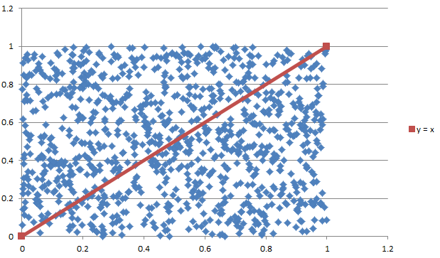 Since we are interested in the area under the curve I coloured all these points in a different colour. 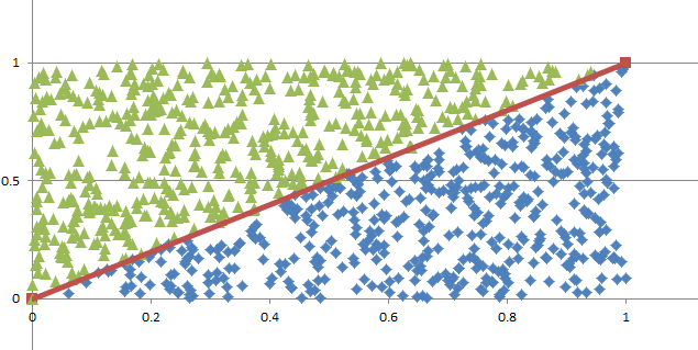 Since we have sampled randomly from the square, we would expect the proportion of points falling below the line will approach the proportion of the area below and above the line. If we examine this ratio we get a value of $ 492 / 1000 $ which is very close to the value of $1/2$ we would expect from analytical methods. Problem 2 - y = x ^ 2 Let's try again on a harder problem. What is the integral of $y = x^2$ between $0$ and $3$? Let's create another graph of this problem: 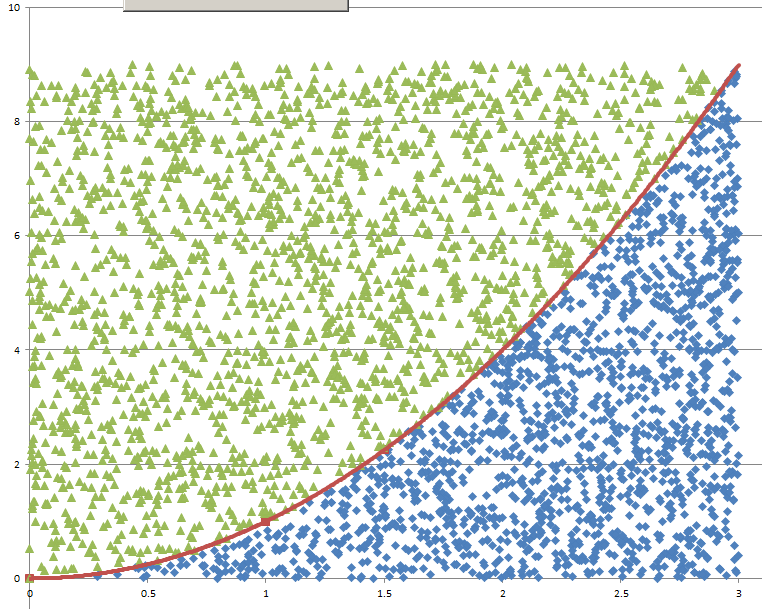 When we look at the results we see that the ratio now is 0.3326, which once again we can see is converging to the answer we expect of 0.3333. I had to bump the number of simulations up to 5000 in this example to get a reasonable fit. Problem 3 - e^(x^2) You might be thinking to yourself at this point - all this is quite interesting but is there any benefit it doing things this way? All we've done so far is check the solutions to intergrals that we already know how to solve! The integral for this problem however is known to have no elementary closed solution. That means that we can't just use A-level maths to calculate the integral. The graph of the function isn't too complicated and looks like this: 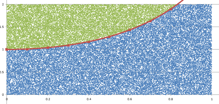 I had to bump up the number of simulations here again to 50,000, but the analysis gave us a figure of 1.46 for the value of the integral. So why does this particular problem matter again? It means that this method is not just an interesting curiosity. But that it actually allows solutions to be calculated for integrals which standard A-level integration techniques don't work for. Uniqueness of Moment Generating Functions18/10/2016
Most undergraduate probability textbooks make extensive use of the result that each random variable has a unique Moment Generating Function. In particular, we can use this result to demonstrate the effect of adding or multiplying random variables. For example, the proof that the sum of two Poisson Random Variables is also a Poisson Random Variable (with mean equal to the sum of the means of the two Poissons) is much easier if we can invoke this result.
Proof for the sum of two Poisson distributions:
Suppose $X$ and $Y$ are independent Poisson Distributions with parameters $\lambda_1$ and $\lambda_2$.
We know that the $MGF$ of a Poisson Distribution with parameter $\lambda$ is $e^{ \lambda ( e^t - 1)) }$.
We can now use the result that:
$MGF_{X+Y} = MGF_X * MGF_Y = e^{ \lambda_1 ( e^t - 1)) } * e^{ \lambda_2 ( e^t - 1)) } = e^{ (\lambda_1 +\lambda_2) ( e^t - 1)) }$
Which is the $MGF$ of a Poisson Distribution with distribution $\lambda_1 + \lambda_2$ proving the result. Do we need a proof? Call me pedantic, but I never liked the fact that this uniqueness result is usually stated without proof. For me, there was always an elegance to a textbook that began with definitions and axioms, and possibly a handful of weak results which were taken as given, and then proved everything required on the way. In my experience Probability and Stats books seem particularly prone to not being self-contained and rigorous in this way. I suspect it has something to do with the fact that probability and stats, if done 100% rigorously, are both extremely technical and difficult! It would be a shame if we had to wait until we had mastered complex analysis and measure theory before we could learn about predicting the number of black and white balls in an urn. (I'm joking there are actually interesting and useful parts to probability once you get past of those boring exercises about urns) I think my discomfort is added to by the fact that there is also something slightly disingenuous in using a very powerful result to prove a fairly trivial special case without really understanding the general result you are using. If you do this too much, you never really understand why anything is true, just that it is true. Not only is this proof not often given, I had to look pretty hard to find it anywhere.. The general proof for all random variables requires either measure theory or complex analysis and is quite involved, therefore I thought I'd just write up the result for discrete random variables. So here is a proof of the uniqueness of $MGFs$ for discrete random variables over the support $\mathbb{N}_0$. Uniqueness of MGFs Suppose $X$ and $Y$ are discrete random variables over $\{ 0 , 1, 2, ... \} $. Further suppose that: That is: Then, $$\sum_{i=0}^{\infty} e^{tx_i} f_X (i) - \sum_{j=0}^{ \infty } e^{tj} f_Y (j) = 0$$ Changing the range for the second sum: $$\sum_{i=0}^{\infty} e^{ti} f_X (i) - \sum_{i=0}^{ \infty } e^{ti} f_Y (i) = 0 $$ Bringing the two sums together: $$\sum_{i=0}^{\infty} ( e^{ti} f_X (i) - e^{ti} f_Y (i) ) = 0 $$ Rearranging: $$\sum_{i=0}^{\infty} e^{ti}(f_X (i) - f_Y (i) ) = 0 $$ We can now think of this as a power series with coefficients: $$g(i) = f_X (i) - f_Y (i)$$ i.e. $$\sum_{i=0}^{\infty} (e^t)^i g(i) = 0 $$ Which allows us to use the result that a power series which is equal to $0$ in some interval (in this case $\mathbb{R}$), must have coefficients equal to $0$ on the interval. To see this, we consider the $nth$ derivative, which allows us to recover the $nth$ coefficient.: $$f^{(n)}(0) = \sum_{k=n}^\infty \frac{k!}{(k-n)!}c_k0^{k-n} = n!c_{n}$$ Which gives us our result since $g(i)=0$ implies that the two functions $f_X$ and $f_Y$ are equal. Chemical Equations and Diophantine Equations17/10/2016
I was reading about SpaceX on Wikipedia the other day, just after they announced their plan to travel to Mars, and about an hour later, as can happen on Wikipedia, I found myself reading about Chemistry and feeling nostalgic about all the subjects that I used to know in detail but now have just a hazy recollection of.
Reading the material on Chemistry got me thinking that there are quite a few similarities between chemical elements and prime numbers. All chemical compounds can be reduced to a combination of chemical elements in a unique way, and all integers can be reduced to a product of prime factors in a unique way. Both serve as the building blocks from which more complicated objects are constructed. What happens if we attempt to formalise this relationship? It turns out we can actually come up with a mathematical process for balancing chemical equations. And this solution is related to the study of mathematical objects called Diophantine equations. What is a Chemical Equation? Let’s start by reviewing what a chemical is. A chemical equation is an equation which defines a chemical reaction. The left hand side has the inputs to the reaction and the right hand side has the outputs. So for example, the process of adding hydrogen and oxygen to create water can be written as: H + O -> H2O This equation though is not balanced. We’ve got two hydrogens on the right, but only one on the left. Therefore there is some information missing. Balancing a Chemical Equation How do we balance a Chemical Equation? We need to define the relative amounts of the inputs and outputs so that the total numbers of each element are the same on both sides of the equation. We do this by writing an integer before each input and an integer before each output to denote the relative amounts of each molecule in the reaction. In the case of the combustion reaction above, we can see by inspection that we need two hydrogen elements and one water element to create a water molecule, that is: 2 H + O = H2O What happens though if we need to balance a more complicated Equation? For example, here is the equation for the combustion of gunpowder: KNO3 + S + C → K2S + N2 + CO2 It is not immediately obvious to me how to balance this equation. It’s not too complicated and could probably be balanced by inspection, but what if the equation was much more complicated? Chemical Elements and Prime Numbers If we take the step of associating a prime number to each element in the equation, for example, let’s make the following associations:
And we also replace the additive notation with a multiplicative notation, then we get the following mathematical equation for the combustion of gunpowder:
$(67*17*(19^3))^a * 47^b * 13^c = ((67^2)*47)^d * (17^2)^e *(13*(19^2))^f$
Equating prime factors on the right and prime factors on the left gives us a system of linear Diophantine equations, one for each prime: a = 2d a = 2e 3a = 2f b = d c = f Diophantine Equations A Diophantine equation is a polynomial equation for which we are only interested in integer solutions. Since a chemical equation must have integer coefficients, the resulting system of linear equations is actually a system of Diophantine equations. So returning to our chemical equation above, we can solve this equation using linear algebra. In this case, I put the system of linear equations into an online calculator, and we find that solutions to this system are of the following form for integers n: a = 2 n b = n c = 3 n d = n e = n f = 3n I used the following online calculator: As we are interested in integer solutions, we need to now find n such that all our coefficients take integer values. In this case, we can take n to be 1 giving us: a = 2 b = 1 c = 3 d = 1 e = 1 f = 3 Putting this back into our equation above we get: 2 KNO3 + S + 3 C → K2S + N2 + 3 CO2 Which we can see is a balanced chemical equation. This process can be extended to balance any chemical equation, no matter how complicated. Using Monte Carlo Methods to estimate Pi13/7/2016 Monte Carlo Methods Monte Carlo methods, named after the area in Monaco famous for it casinos, are a collection of mathematical methods that use repeatedly sampling of random numbers to solve mathematical problems. They are commonly used to simplify problems that would otherwise be impossible or too time consuming to solve if we were forced to use analytical methods. An example Suppose we are given the option of playing the following game in a casino: The game costs £5 per play. The game involves you rolling 10 dice. If the sum of the dice is greater than 45, you win £10, otherwise you don't win anything. Should you play this game? Off the top of my head, I've got no idea whether this is good value or not. Given we are in a casino, I'm going to guess we would lose money over the long run, but what if we wanted to know for sure? We could work out the answer analytically, we could say things like the probability of rolling a 45 using 7 dice is impossible, but using 8 dice it is.... then work recursively from there and it would take a long time and would be quite tedious. An alternative approach would be to set up a model that would simulate the playing of this game, run the model a few thousand times (which should take seconds) and then see what the long term position is when we average across all the games. Much more interesting. I quickly set up a test of the game, and it turns out it is very bad value. On average we would expect to lose about £4.60 every time we play! The interesting point though is that it took me a couple of minutes to work this out, compared to the hours it would have taken me to calculate it analytically. Monte Carlo Methods in insurance Monte Carlo methods are also commonly used in insurance. For example, in reinsurance pricing, when attempting to find an expected value for a loss to an excess of loss layer we may have a good idea of the size and frequency of the ground up losses, say we know that the frequency of losses is distributed according to a Poisson distribution with a known parameter, and the severity of the losses is distributed according to a Log-normal distribution with known parameters. What can we say about the loss to the layer however? It may be theoretically possible to derive this analytically in some cases, but generally this will be too time consuming and may not even be possible. A Monte Carlo approach, like the dice game earlier, involves repeatedly playing the game, we imagine that we write the contract and we then sample values from the frequency and severity distributions to generate sample loss amounts, we can then apply all the contract details to these generated loss amounts. This process of sampling is repeated tens of thousands of times and by averaging across all our simulations we can derive estimates of the expected loss to the layer or any other piece of information we may be interested in. Other uses of Monte Carlo Methods We can also use Monte Carlo methods in other situations where we wish to estimate a value where analytical methods may fall short.
One example of this is in calculating the value of $\pi$. We use the fact that the area of a unit circle is $\pi$. If we imagine the unit circle sitting inside a unit square, then the area of the unit square is 4, and the ratio of the area inside the circle to the area inside the square is $\pi : 4$. Here is some Octave code to generate a picture:
hold on x = -1:0.001:1; y = (1 - x.^2).^0.5; plot(x,y,'linewidth',2); plot(x,-y,'linewidth',2); plot([1,-1],[-1,-1],'linewidth',2); plot([-1,-1],[-1,1],'linewidth',2); plot([-1,1],[1,1],'linewidth',2); plot([1,1],[1,-1],'linewidth',2); 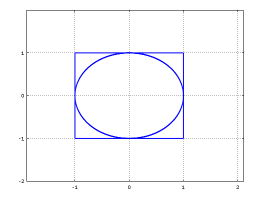
Now suppose we were to sample random points from within the unit square. We can easily check whether a point is inside the circle or outside using the equation of the circle, i.e.:
$ x^2 + y^2 <= 1$
For points that fall inside the circle.
Given the ratio of the circle to the square, we would expect the proportion of randomly selected sample points which end up inside the circle to approach $\pi /4$. And we can therefore use this value to estimate $\pi$.
With the following Octave code we get a sense of what is happening:
hold on x = -1:0.001:1; y = (1 - x.^2).^0.5; plot(x,y,'linewidth',2); plot(x,-y,'linewidth',2); plot([1,-1],[-1,-1],'linewidth',2); plot([-1,-1],[-1,1],'linewidth',2); plot([-1,1],[1,1],'linewidth',2); plot([1,1],[1,-1],'linewidth',2); SampleSize = 1000; Sample = unifrnd (-1, 1, 2, SampleSize); Results = 1:SampleSize; for i = 1:SampleSize Results(i) = Sample(1,i).^2 + Sample(2,i).^2; endfor for i = 1:SampleSize if Results(i) <= 1 plot(Sample(1,i),Sample(2,i),'k'); else plot(Sample(1,i),Sample(2,i),'r'); endif endfor 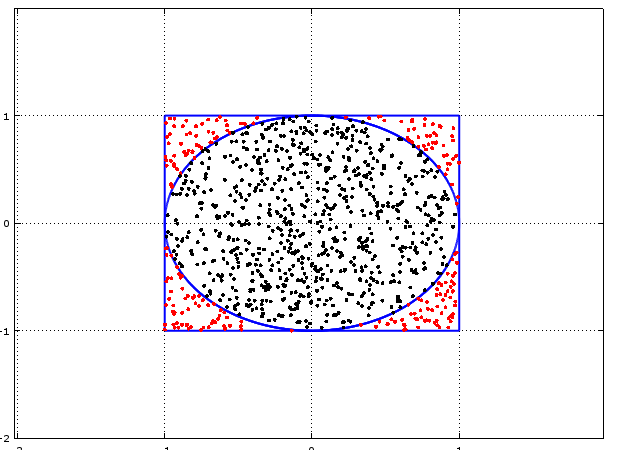
If we count the number of black dots and divide it by the total number of dots then this ratio will allow us to estimate $\pi$.
The final code is: SampleSize = 100000; Sample = unifrnd (-1, 1, 2, SampleSize); Results = 1:SampleSize; for i = 1:SampleSize Results(i) = Sample(1,i).^2 + Sample(2,i).^2; endfor Pi = 0; for i = 1:SampleSize; if Results(i) <= 1 Pi = Pi + 1/SampleSize; endif endfor 4*Pi Why not give it a go yourself!
Why do we use the Poisson Distribution as the default distribution for modelling Claims Frequency for an insurance portfolio?
Why do we even have a default? When we are setting up a frequency-severity model to model claims from a insurance portfolio, we will normally approach the fitting of a frequency distribution and the fitting of the severity distribution quite differently. For the frequency distribution the standard approach is to attempt to fit a Poisson distribution, and only look at other distributions if the Poisson is not a good fit (even then we normally limit our search to Negative Binomial, and maybe Binomial at a stretch) When we fit a severity model however, we will often fit quite a large range of different continuous probability distribution to the empirical Claim Severity CDF using some sort of curve fitting software and then select the most appropriate curve. Some Distributions are used more often than others, for example, LogNormal, Pareto, Weibull are all common curves to use, but there is no single curve that we would assume the severity distribution conforms to by default. So why is a Poisson distribution a natural distribution to use to model claims frequency? And why is there no 'natural' distribution for claim severity? In this post I thought I would write up an interesting result that shows that a counting distribution which has a number of basic properties will be distributed with a Poisson distribution. We will then be able to see that are reasonable assumptions to make about Claims Frequency for an insurance portfolio.
Poisson Distribution
Before working through this result, here are a list of additional properties the Poisson Distribution has which make it easy to work with:
$$ N \sim Poi( \lambda )$$
Then
The Result
Let $A(t)$ for ($t >0$) denote the the number of claims in the interval $[0,t]$. With $A(0) = 0$.
Suppose:
$$P( A(t + \delta t) - A(t) \geq 2 ) = o( \delta t)$$
The Proof
Define $P_n (t) = P( A(t) = n ) $
We then examine the change in $P_n(t)$ over a time period $\delta t$ and then take the limit as $\delta t$ approaches $0$.
for $n > 0$: $$P_n(t + \delta t) = P_n(t)(1 − \lambda \delta t) + P_{n−1} (t) \lambda \delta t + o( \delta t) $$ for $n = 0$: $$P_0(t + \delta t) = P_0(t)(1 − \lambda \delta t) + o( \delta t)$$
This follows from the facts that there are two distinct ways for $n$ claims to happen in a time period $t + \delta t$. Either we get $n$ claims in time $t$ and no claims in $\delta t$, or $n-1$ claims in time $t$ and one claim in $\delta t$.
We can rewrite these equations as: for $n > 0$: $$\frac { Pn(t + δt) − Pn(t)}{\delta t} = \frac {−P_n(t)( \lambda \delta t) + P_{n−1}(t) \lambda \delta t + o(\delta t)} { \delta t}$$ for $n = 0$: $$\frac {P_0 ( t + \delta t) − P_0(t)} {\delta t} = \frac {P_0(t)(− \lambda \delta t) + o(\delta t) } {\delta t}$$ Now take the limit as $\delta \to 0$ which gives: for $n>0$: $$\frac { d P_n (t)} {dt} = − \lambda P_n(t) + \lambda P_{n−1}(t)$$ for $n=0$: $$\frac {d P_0 (t)} {dt} = - \lambda P_0 (t)$$ From inspection we can see that $P_0 (t) = e^{ {- \lambda} }$ The proof for the general case can easily be shown with induction. We therefore see that $P_n$ has a Poisson distribution.
Poisson as the natural distribution
So we see that, in so far as insurance claims occur in line with the assumptions (independently over the time interval, and only one at a time) we can expect the claims frequency to have a Poisson Distribution. In addition, the Poisson Distribution has a number of properties which make it easy to work with - having a single parameter, having simple formulas for the mean and variance, etc. Therefore, whenever we are fitting a claim frequency model, we will almost always try the Poisson Distribution first.
In Options, Futures and Other Derivatives, Chapter 10, Hull derives lower bounds for option prices for European put and call options for dividend paying stocks.
The result in Hull: For a call option:
$c_0 \geq S_0 - K e^{-rT}$
For a put option:
$p_0 \geq K e^{-rT} - S_0 $
And he also derives upper bounds for European put and call options for non-dividend paying stocks. For a call option:
$c_0 \leq S_0$
For a put option:
$p_0 \leq K e^{-rT}$
But he doesn't derive upper bounds for European put and call options for dividend paying stocks. And for call options this gives us a tighter upper bound. Also I wasn't able to find this bound online for some reason, it's almost like everyone is just copying these results from other people and not actually deriving them themselves. The new Result Let $S_T$ = price of the stock at time $T$. $K$ = Strike price of the option $T$ = Maturity of the option $q$ = dividend yield of the stock $c_t$ = price of the call option at time $t$. $max(S_T,K) \leq S_T + K$ $max(S_T,K) - K \leq S_T$ $max(S_T-K,0) \leq S_T$ $c_T \leq S_T$ Then by a no arbitrage argument: $c_0 \leq S_0 e^{-qT}$ Which is a tighter upper bound than for a non-dividend paying stock. LIBOR Bond Pricing3/1/2016
I was working through Hull's Options, Futures and other Derivatives when Hull states that the price of a Bond paying semi annual coupons in line with six month LIBOR, and discounted using a six month LIBOR discount rate is par. To me this statement seems like it's probably true but I wasn't 100%. I couldn't find the proof online, but it turns out that it is true, here is my derivation.
Proof by induction:
Base case: $n=1$ value(n year bond) $= $PAR $ = \sum\limits_{i=1}^{2n-1}\frac{(PAR)R/2}{(1+R/2)^i} + \sum\limits_{i=2n}^{2(n+1)-1}\frac{(PAR)R/2}{(1+R/2)^i}$ $+ \frac{PAR(1+R/2)}{(1+R/2)^{(2(n+1))}} + \left(\frac{(PAR)(1+R/2)}{(1+R/2)^{2n}}-\frac{(PAR)(1+R/2)}{(1+R/2)^{2n}}\right)$ Rearranging:$ = \left(\sum\limits_{i=1}^{2n-1}\frac{(PAR)R/2}{(1+R/2)^i} + \frac{(PAR)(1+R/2)}{(1+R/2)^{2n}}\right) + \sum\limits_{i=2n}^{2(n+1)-1}\frac{(PAR)R/2}{(1+R/2)^i}+ \frac{PAR(1+R/2)}{(1+R/2)^{(2(n+1))}} -\frac{(PAR)(1+R/2)}{(1+R/2)^{2n}}$ Then using the fact that a n year bond is priced at PAR:$ = PAR + \sum\limits_{i=2n}^{2(n+1)-1}\frac{(PAR)R/2}{(1+R/2)^i}+ \frac{PAR(1+R/2)}{(1+R/2)^{(2(n+1))}} -\frac{(PAR)(1+R/2)}{(1+R/2)^{2n}}$ No we just take the PAR outside and cancel out to 1.$ = PAR\left(1 + \sum\limits_{i=2n}^{2(n+1)-1}\frac{R/2}{(1+R/2)^i}+ \frac{(1+R/2)}{(1+R/2)^{(2(n+1))}} -\frac{(1+R/2)}{(1+R/2)^{2n}}\right)$ $ = PAR\left(1 + \frac{R/2}{(1+R/2)^{(2n)}} + \frac{R/2}{(1+R/2)^(2n+1)}+ \frac{1}{(1+R/2)^{(2n+1)}} -\frac{1}{(1+R/2)^{2n-1}}\right)$ $ = PAR\left(1 + \frac{R/2}{(1+R/2)^{(2n)}} + \left(\frac{R/2}{(1+R/2)^(2n+1)}+ \frac{1}{(1+R/2)^{(2n+1)}}\right) -\frac{1}{(1+R/2)^{2n-1}}\right)$ $ = PAR\left(1 + \frac{R/2}{(1+R/2)^{(2n)}} + \frac{1+ R/2}{(1+R/2)^(2n+1)}+ -\frac{1}{(1+R/2)^{2n-1}}\right)$ $ = PAR\left(1 + \frac{R/2}{(1+R/2)^{(2n)}} + \frac{1}{(1+R/2)^(2n)}+ -\frac{1}{(1+R/2)^{2n-1}}\right)$ $ = PAR\left(1 + \left(\frac{R/2}{(1+R/2)^{(2n)}} + \frac{1}{(1+R/2)^(2n)} \right)+ -\frac{1}{(1+R/2)^{2n-1}}\right)$ $ = PAR\left(1 + \frac{1 + R/2}{(1+R/2)^{(2n)}} -\frac{1}{(1+R/2)^{2n-1}}\right)$ $ = PAR\left(1 + \frac{1}{(1+R/2)^{(2n -1)}} -\frac{1}{(1+R/2)^{2n-1}}\right)$ $ = PAR$
When you order at 5 guys burgers (which you should if you haven't because they are amazing) you are given a ticket between 1 and 100 which is then use to collect your order. Last time I was there my friend suggested trying to collect all 100 tickets. The question is:
Assuming you receive a random ticket number between 1 and 100 inclusive on every visit. On average, how many visits would it take to collect all 100 tickets? Solution:
Define $S$ to be a random variable which counts the number of purchases required to get all 100 tickets. Then we are interested in $\mathbb{E} [S]$
To help us analyse $S$ we need to define another collection of random variables. Let $X_i$ denote the number of purchases required to get the $ith + 1$ ticket given we have already collected $i$ tickets. So if we have collected 2 tickets (say ticket number 33 and ticket number 51) and the next two tickets we get are 33 and 81, then $X_2 = 2$ because it took us 2 attempts to get a new unique ticket. We can actually view $S$ as the sum of these $X_i$, i.e. $S = \sum\limits_{i=1}^{100}X_i$ (to see that this is the case the number of visit it takes to collect all 100 tickets will be the number of visits to collect the first ticket plus the number of visits to collect the 2nd unique ticket, and so on) There are two further observations that we need to make before deriving the solution. Firstly, each $X_i$ is independent of $\sum\limits_{k=1}^{{i-1}}X_i$. Secondly, each $X_i$ is actually distributed as a Geometric Distribution where:
$P( X_i = k ) = \frac{i-1}{100}^{k-1} \frac{101-i}{100}$
Giving us: $\mathbb{E} [ S ] = \mathbb{E} [ \sum\limits_{k=1}^{100} X_i ] = \sum\limits_{k=1}^{100} \mathbb{E} [X_i ] = \sum\limits_{k=1}^{100} \frac{100}{101-i} = 100 \sum\limits_{k=1}^{100} \frac{1}{101-i} = 100 \sum\limits_{k=1}^{100} \frac{1}{i}$ |
AuthorI work as an actuary and underwriter at a global reinsurer in London. Categories
All
Archives
April 2024
|
 RSS Feed