What is a 'Net' Quota Share?7/10/2022 I recently received an email from a reader asking a couple of questions : "I'm trying to understand Net vs Gross Quota shares in reinsurance. Is a 'Net Quota Share' always defining a treaty where the reinsurer will pay ceding commissions on the Net Written Premium? ... Are there some Net Quota Shares where the reinsurer caps certain risks (e.g. catastrophe)?" It's a reasonable question, and the answer is a little context dependent, full explanation given below.  Source: https://unsplash.com/@laurachouette, London
(As an aside, in the last couple of weeks, the UK has lurched from what was a rather pleasant summer into a fairly chilly autumn, to mirror this, here's a photo of London looking a little on the grey side.) I wrote a quick script to backtest one particular method of deriving claims inflation from loss data. I first came across the method in 'Pricing in General Insurance' by Pietro Parodi [1], but I'm not sure if the method pre-dates the book or not. In order to run the method all we require is a large loss bordereaux, which is useful from a data perspective. Unlike many methods which focus on fitting a curve through attritional loss ratios, or looking at ultimate attritional losses per unit of exposure over time, this method can easily produce a *large loss* inflation pick. Which is important as the two can often be materially different. 
Source: Willis Building and Lloyd's building, @Colin, https://commons.wikimedia.org/wiki/User:Colin
An Actuary learns Machine Learning - Part 13 - Kaggle Tabular Playground Competition - June 221/7/2022 
In which we recreate the previous analysis, but in Python this time. And then add a new submission using Mean rather than median to impute missing values. Source: https://somewan.design An Actuary learns Machine Learning - Part 12 - Kaggle Tabular Playground Competition - June 2224/6/2022  In which we start a new Kaggle competition, submit a dummy attempt, and then build a very basic Excel model to establish a baseline for future progress. Source: https://somewan.design Quota Share contracts generally deal with acquisition costs in one of two ways - premium is either ceded to the reinsurer on a ‘gross of acquisition cost’ basis and the reinsurer then pays a large ceding commission to cover acquisition costs and expenses, or premium is ceded on a ‘net of acquisition’ costs basis, in which case the reinsurer pays a smaller commission to the insurer, referred to as an overriding commission or ‘overrider’, which is intended to just cover internal expenses. Another way of saying this is that premium is either ceded based on gross gross written premium, or gross net written premium. I’ve been asked a few times over the years how to convert from a gross commission basis to the equivalent net commission basis, and vice versa. I've written up an explanation with the accompanying formulas below.  Source: @ Kuhnmi, Zurich
Investopedia defines TBVPS to be: "Tangible book value per share (TBVPS) is the value of a company’s tangible assets divided by its current outstanding shares." [1] I'm pretty sure this is incorrect. or at best misleading!  Canary Wharf, source: https://commons.wikimedia.org/wiki/User:King_of_Hearts
Downloading data from Wiki22/4/2022 Did you know about this cool tool, which allows you to download data from a Wikipedia table as a csv: wikitable2csv.ggor.de/ How to interpolate in a Spreadsheet15/4/2022 Here's a useful trick that you might not have seen before. Suppose we have some data with includes rows with values missing, then we can use the below formula to apply linear interpolate to fill in the missing datapoints, without having to laboriously type in the interpolation formula long hand (which I used to do all the time) 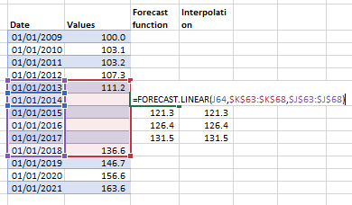
I wrote a python script which uses Selenium to scrape the predictions for Fed rate movements from the CME FedWatch tool.
www.cmegroup.com/trading/interest-rates/countdown-to-fomc.html#resources The tool works by converting the price of a 30 day Fed Fund future into an implied probability of a given range of yields. The CME website embeds the output in a something called an 'iframe', which I had never heard of before, and the iframe then contains a dashboard powered by something called Quikstrike. It took me a while to figure out how to switch focus to the iframe, as you can't simply reference elements inside the iframe without first switching focus. The script below may not look too complicated, but believe me, it took a while to write. 
Old Federal Reserve building Philadelphia, Source: https://commons.wikimedia.org/wiki/User:Beyond_My_Ken
The official Microsoft documentation for the Excel Forecast.ETS function is pretty weak [1]. Below I’ve written a few notes on how the function works, and the underlying formulas.  Source: Microsoft office in Seattle, @Coolcaesar, https://en.wikipedia.org/wiki/File:Building92microsoft.jpg
It's still very early days to understand the true fallout from Russia's invasion of Ukraine, but I thought it would be interesting to tally a few of the estimates for the insured loss we've seen so far, all of the below come from the Insider. Please note, I'm not endorsing any of these estimates, merely collating them for the interested reader!  Kiv Perchersk Lavra Monastery, Kyiv. @Andriy155
Aggregating probability forecasts18/3/2022 There's some interesting literature from the world of forecasting and natural sciences on the best way to aggregate predictions from multiple models/sources. For a well-written, moderately technical introduction, see the following by Jaime Sevilla: forum.effectivealtruism.org/posts/sMjcjnnpoAQCcedL2/when-pooling-forecasts-use-the-geometric-mean-of-odds Jaime’s article suggests a geometric mean of odds as the preferred method of aggregating predictions. I would argue however that when it comes to actuarial pricing, I'm more of a fan of the arithmetic mean, I'll explain why below.  Python script - PredictIt API11/3/2022
I wrote a quick Python script to download the latest odds from PredictIt, and then output to an Excel file. I've pasted it below as an extract from a Jupyter notebook:
PredictIt is an online prediction website, mainly focused on Political events: www.predictit.org/ I think it's great that PredictIt allow access like this, before I realised the API exists I was using Selenium to scrape the info through Chrome, which was much slower to run, and also occasionally buggy. Cefor Exposure Curves - follow up7/3/2022 The Cefor curves provide quite a lot of ancillary info, interestingly (and hopefully you agree since you're reading this blog), had we not been provided with the 'proportion of all losses which come from total losses', we could have derived it by analysing the difference between the two curves (the partial loss and the all claims curve) Below I demonstrate how to go from the 'partial loss' curve and the share of total claims % to the 'all claims' curve, but you could solve for any one of the three pieces of info given two of them using the formulas below.  Source: Niels Johannes https://commons.wikimedia.org/wiki/File:Ocean_Countess_(2012).jpg
Cefor Exposure Curves3/3/2022 I hadn't see this before, but Cefor (the Nordic association of Marine Insurers), publishes Exposure Curves for Ocean Hull risks. Pretty useful if you are looking to price Marine RI. I've included a quick comparison to some London Market curves below and the source links below. 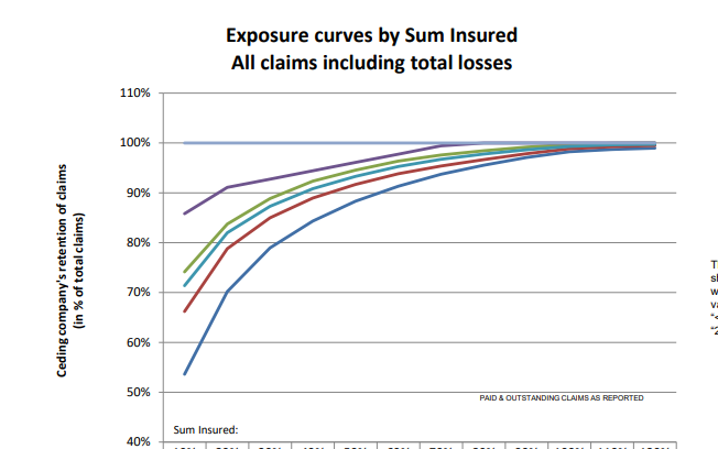 |
AuthorI work as an actuary and underwriter at a global reinsurer in London. Categories
All
Archives
April 2024
|
 RSS Feed