Inflation modelling - median of top 10 losses, with additional years of data

24/7/2023

In my last couple of post on estimating claims inflation, I’ve been writing about a method of deriving large loss inflation by looking at the median of the top X losses over time. You can read the previous posts here:

Part 1: www.lewiswalsh.net/blog/backtesting-inflation-modelling-median-of-top-x-losses
Part 2: www.lewiswalsh.net/blog/inflation-modelling-median-of-top-10-losses-under-exposure-growth

One issue I alluded to is that the sampling error of the basic version of the method can often be so high as to basically make the method unusable. In this post I explore how this error varies with the number of years in our sample, and try to determine the point at which the method starts to become practical.

Photo by Jøn

Just to refresh, we saw in the previous post that when calculating the inflation using 10 years of loss data, that our central estimate was 5%, but that the standard deviation of our estimate was around 2.5%. This is very high! Assuming a normal distribution of error, and using a 95% threshold, i.e. bounding by 2 standard deviations, we could estimate our true inflation rate to be in the range [0%,10%] with a 95% confidence. For most practical purposes, this is basically useless. Many risks you might price would look very attractive at 3% inflation and down right crazy at 8% inflation.

What can we do to improve the standard deviation of the method?

Today we're going to examine the effect of including additional years of loss data in the calculation. Last time we used 10 years, now we're going to look at varying n = number of years, from n=2 to n=50.

Let’s amend our code to add an additional loop which runs from 2 to 50 years of loss data. We'll also record the standard deviations as we go, and then output a graph at the end. As before, we've set the true inflation rate to 5%, and we are not using any exposure adjustments.

Here’s our updated code:

In [1]:

import numpy as np
import pandas as pd
import scipy.stats as scipy
import matplotlib.pyplot as plt
from math import exp
from math import log
from math import sqrt
from scipy.stats import lognorm
from scipy.stats import poisson
from scipy.stats import linregress

import time

In [2]:

Distmean = 1500000.0
DistStdDev = Distmean*1.5
AverageFreq = 100
years = 20
ExposureGrowth = 0 #0.02

Mu = log(Distmean/(sqrt(1+DistStdDev**2/Distmean**2)))
Sigma = sqrt(log(1+DistStdDev**2/Distmean**2))

LLThreshold = 1e6
Inflation = 0.05

s = Sigma
scale= exp(Mu)

results=["Distmean","DistStdDev","AverageFreq","years","LLThreshold","Exposure Growth","Inflation"]

In [4]:

AllMean = []
AllStdDev = []

for numyears in range(2,51):

    MedianTop10Method = []
    AllLnOutput = []
    years = numyears
    #print(years)
    
    for sim in range(750):
    
        SimOutputFGU = []
        SimOutputLL = []
        year = 0
        Frequency= []
        for year in range(years):
            FrequencyInc = poisson.rvs(AverageFreq*(1+ExposureGrowth)**year,size = 1)
            Frequency.append(FrequencyInc)
            r = lognorm.rvs(s,scale = scale, size = FrequencyInc[0])
            r = np.multiply(r,(1+Inflation)**year)
            r = np.sort(r)[::-1]
            r_LLOnly = r[(r>= LLThreshold)]
            SimOutputLL.append(np.transpose(r_LLOnly))
            
        SimOutputLL = pd.DataFrame(SimOutputLL).transpose()    
        a = np.log(SimOutputLL.iloc[5])
        AllLnOutput.append(a)
        b = linregress(a.index,a).slope
        MedianTop10Method.append(b)
    
    AllLnOutputdf = pd.DataFrame(AllLnOutput)
    
    dfMedianTop10Method= pd.DataFrame(MedianTop10Method)
    dfMedianTop10Method['Exp-1'] = np.exp(dfMedianTop10Method[0]) -1
    AllMean.append(np.mean(dfMedianTop10Method['Exp-1']))
    AllStdDev.append(np.std(dfMedianTop10Method['Exp-1']))
    
plt.plot(AllStdDev)
plt.xlabel("Years of loss data")
plt.ylabel("Standard deviation")
plt.show()

In [ ]:

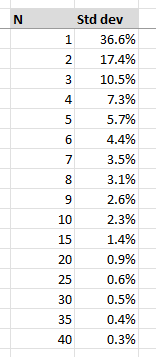
And here is the numerical output in a table:

We can see that as the number of years included increases, that the standard deviation falls. So far so good. Recall that in our previous post, with 10 years of data the standard deviation was around 2.5%, and in the table above, we can see a value of 2.3%. So the code is consistent with our previous modelling. Bounding the 5% central estimate by 2 standard deviations got us our range of [0,10%]. Now, with 20 years of loss data instead, our standard deviation drops to around 1%, and we’d have a range of [3%,7%] at a 95% threshold. Still quite wide, but definitely an improvement.

What if we want to get our 95% range to 1% either side? Then based on the table above, we'd need 30 years of loss data. I'd say 1% inflation either way as a bound is starting to get practical now. If I'm modelling a risk and a 2% swing in inflation is completely blowing me out of the water, then I've got more issues than just how to estimate the inflation in the first place, I should probably revisit my modelling and see why it's so sensitive.

What speed does the deviation drop at?

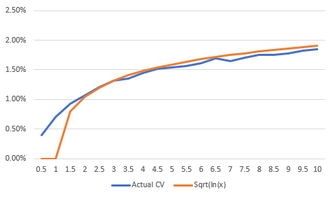
I initially thought it looked like a x^-2, but its actually a bit slower than that. The best fit I could find was using the curve $a x ^{-b}$. with a=0.45, and b = 1.34. i.e. it decays at a degree $-1.34$. Here is the fit against actual for years 10 onwards.

Conclusions

The results above do mean we need a decent number of years to reduce the standard deviation much further. For example, we saw that we needed 30 years of data to get to a range of 1% either side at a 95% confidence level.

Does this analysis then solve our problem? Well, there’s still a couple of issues. Firstly, we require a large number of years of loss data to start getting a useable estimate, but what if we don’t have this data? The second problem is a bit more pernicious, what if inflation has changed materially over the last 30 years? Even if we get a solid estimate of the inflation over the last 30 years, we're probably most interested in applying it to the loss experience from the last 10 years of so. We really need a method that gives meaningful estimates using a smaller dataset. This is particularly relevant if looking at US casualty, due to the wave of social inflation starting circa 2015. Our method here, which suggests we look at 30 years of loss history, is not really going to be able to identify this trend.

I think there's still positives to be gleaned from these results, we've seen that across a long enough time horizon, these methods do start to produce credible estimates. So at least we can make statements like - the long term average inflation for US casualty is x - with some level of confidence. We can then start asking ourselves - okay, is the most recent 10 years of inflation better or worse than the long term average, and that can inform our pick for the 10 year window.

What are our next steps?

I am interested in ways that we can improve this method, but before we start going much further, I want to make sure the approach I'm using above is robust across multiple datasets. So I'm planning on I'm repeating the above steps but varying the loss distribution (rather than just using lognormal) and also varying the average mean and standard deviation.

When we do look to improve the method, the first thing I'd like to investigate is the choice of metric we are basing the inflation estimate on. If we just think about how our method works, one of the first things we do is group our losses by year, and then immediately ignore almost all our loss data other than the N-th largest loss. Surely, chucking out most of your data, can't be the most effective way to model a problem?

Inflation modelling - median of top 10 losses, with additional years of data

Leave a Reply.

Author

Sign up to get updates when new posts are added

Categories

Archives