Inflation modelling - median of top 10 losses, under exposure growth

I previously wrote a post in which I backtested a method of deriving large loss inflation directly from a large loss bordereux. This post is an extension of that work, so if you haven't already, it's probably worth going back and reading my original post. Relevant link:
www.lewiswalsh.net/blog/backtesting-inflation-modelling-median-of-top-x-losses
​
In the original post I slipped in the caveat that that the method is only unbiased if the underlying exposure doesn’t changed over the time period being analysed. Unfortunately for the basic method, that is quite a common situation, but never fear, there is an extension to deal with the case of changing exposure.

Below I’ve written up my notes on the extended method, which doesn't suffer from this issue. Just to note, the only other reference I’m aware of is from the following, but if I've missed anyone out, apologies! [1]

St Paul's, London. Photo by Anthony DELANOIX

​​Let’s review the old code first and see where it breaks down. As before, we simulate 10 years of individual losses from a Poisson-Lognormal model, and then apply 5% inflation pa. Let’s now also apply an ‘ExposureGrowth’ factor, which grosses up the average annual frequency prior to simulating the Poisson variable.

(for some reason, I can only embed one Jupyter notebook per page, so the below is just an image, but the second box below has code that can actually be copied)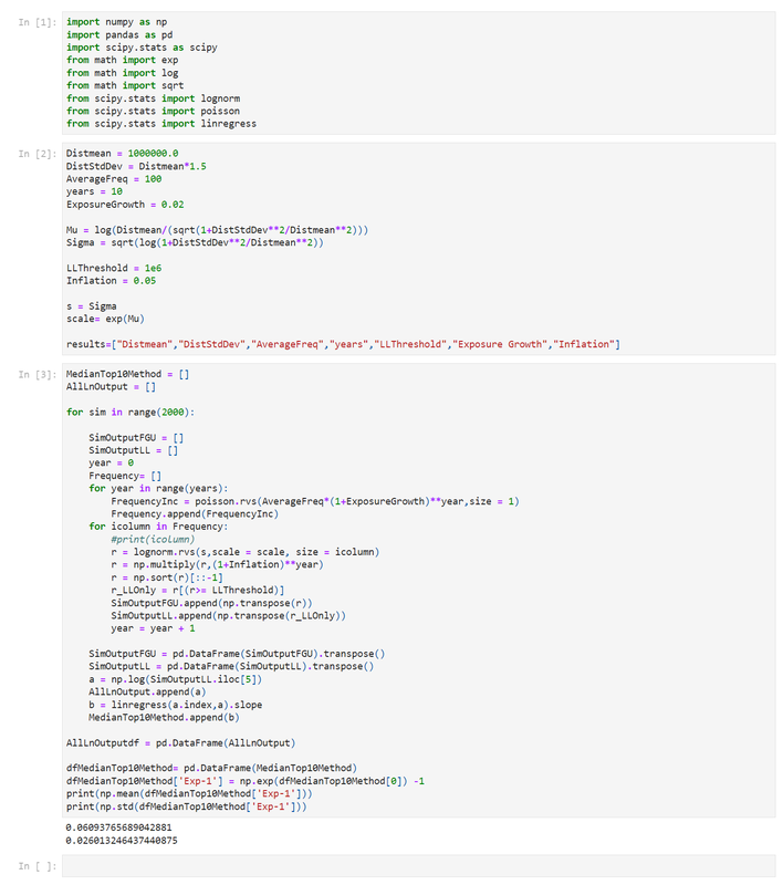

​​We can see that now that we’ve input the exposure growth at 2%, we've still got inflation at 5%, but now the model is producing an inflation estimate of 6.1%. So the method is being thrown off.

So what’s the intuition here?

The basic method works by inferring the inflation by looking at the increase in the 5th largest loss in each year. By using the 5th largest, we effectively circumvent any threshold effects (see the following for example [2]). And based on the set-up of the problem, the only other effect which acts to increase the size of the 5th largest loss over time is severity inflation. However, if we have more losses overall, i.e. under the assumption of exposure increase, then this also acts to push up the size of the 5th largest loss, hence why the method is being thrown off.

How do we fix this?

To adjust for this, instead of always looking at the 5th largest loss, we will instead try to track the same percentile of the loss distribution, adjusting for what we know about the increase in FGU losses.

Note that in the version of the method I've given below, we adjust in line with the actual number of losses in each year (akin to being given info on FGU claim statistics by year). We may not always be given this info however. If instead we only have the change in the exposure metric over time, then we would adjust for the change in *expected* FGU losses over time rather than *actual* FGU losses. Where expected FGU losses would be assumed to increase in proportion to the increase in exposure metric. Note that either adjustment should work in so far as they will produce an unbiased estaimte, but we will have a higher sampling error if we only know the exposure metric vs knowing the change in actual FGU losses.

If we don't know either of these two pieces of information (FGU losses or exposure metric), then there's nothing we can do to salvage the method, as we would have an effect (exposure increase leading to increase in FGU losses) which is pushing up the size of the 5th largest claim, but no way of estimating the size of the effect and thereby removing it.

Here is the amended code :

In [1]:

import numpy as np
import pandas as pd
import scipy.stats as scipy
from math import exp
from math import log
from math import sqrt
from scipy.stats import lognorm
from scipy.stats import poisson
from scipy.stats import linregress

In [2]:

Distmean = 1000000.0
DistStdDev = Distmean*1.5
AverageFreq = 100
years = 10
ExposureGrowth = 0.02

Mu = log(Distmean/(sqrt(1+DistStdDev**2/Distmean**2)))
Sigma = sqrt(log(1+DistStdDev**2/Distmean**2))

LLThreshold = 1e6
Inflation = 0.05

s = Sigma
scale= exp(Mu)

results=["Distmean","DistStdDev","AverageFreq","years","LLThreshold","Exposure Growth","Inflation"]

In [4]:

MedianTop10Method = []
AllLnOutput = []

for sim in range(10000):

    SimOutputFGU = []
    SimOutputLL = []
    Frequency= []
    for year in range(years):
        FrequencyInc = poisson.rvs(AverageFreq*(1+ExposureGrowth)**year,size = 1)
        Frequency.append(FrequencyInc)
        r = lognorm.rvs(s,scale = scale, size = FrequencyInc[0])
        r = np.multiply(r,(1+Inflation)**year)
#        r = np.sort(r)[::-1]
        r_LLOnly = r[(r>= LLThreshold)]
        r_LLOnly = np.sort(r_LLOnly)[::-1]
#        SimOutputFGU.append(np.transpose(r))
        SimOutputLL.append(np.transpose(r_LLOnly))
        
    SimOutputFGU = pd.DataFrame(SimOutputFGU).transpose()
    SimOutputLL = pd.DataFrame(SimOutputLL).transpose()    
    SimOutputLLRowtoUse = []
    for iColumn in range(len(Frequency)):
        iRow = round(5 *Frequency[iColumn][0]/AverageFreq)
        SimOutputLLRowtoUse.append(SimOutputLL[iColumn].iloc[iRow])
    SimOutputLLRowtoUse  = pd.DataFrame(SimOutputLLRowtoUse)
    a = np.log(SimOutputLLRowtoUse)
    AllLnOutput.append(a[0])
    b = linregress(a.index,a[0]).slope
    MedianTop10Method.append(b)

AllLnOutputdf = pd.DataFrame(AllLnOutput)

dfMedianTop10Method= pd.DataFrame(MedianTop10Method)
dfMedianTop10Method['Exp-1'] = np.exp(dfMedianTop10Method[0]) -1
print(np.mean(dfMedianTop10Method['Exp-1']))
print(np.std(dfMedianTop10Method['Exp-1']))

0.05063873870883602
0.024638292351351756

In [ ]:

We can see that when we run this we now get an answer of 5.06%, which is almost exactly back to the 5% we  were expecting. I don’t think the extra 0.06% is related to lack of simulations, I tried upping the sims and it still seems to want to sit just above 5%. I think what is happening is that since we are using the round function to move to the closest discrete loss from the 5th loss, there is probably some bias towards still using a higher percentile than is strictly warranted. So a further improvement would be to interpolate to the exact percentile we are interested in. But since we are already producing an average output very close to the correct value, and much much closer than the one standard deviation, I think it would be a bit unreasonable to quibble over the last 0.1% given the pretty large sampling error that still remains.
 
Summary
We can see that we now have a method that produces unbiased estimates of large loss inflation, even under changes in underlying exposure, isn't that cool? One big problem that still exists however is our standard deviation is still very high. To such an extent that I'd basically call the method unusable in it's current form, against these particular parameters I've used to simulate the data. I'm planning to continue this series of posts to explore a few ways of trying to make the method more accurate, and therefore more practical.

[1] Parodi, P (2014). Pricing in General Insurance.
[2] Brazauskas, V., Jones, B., & Zitikis, R. (2015). Trends in disguise. Annals of Actuarial Science, 9(1), 58-71. doi:10.1017/S1748499514000232