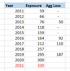
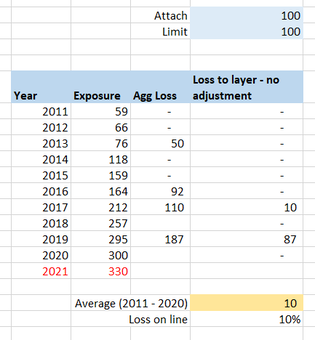
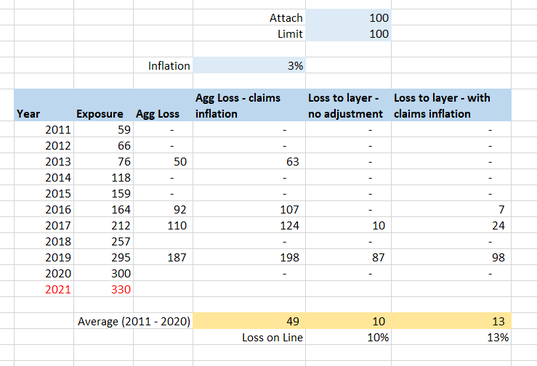
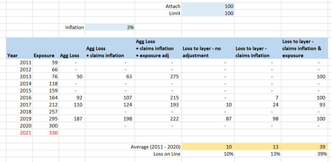
Exposure inflation vs Exposure inflation

The term exposure inflation can refer to a couple of different phenomena within insurance. A friend mentioned a couple of weeks ago that he was looking up the term in the context of pricing a property cat layer and he stumbled on one of my blog posts where I use the term. Apparently my blog post was one of the top search results, and there wasn’t really much other useful info, but I was actually talking about a different type of exposure inflation, so it wasn’t really helpful for him.
​
So as a public service announcement, for all those people Googling the term in the future, here are my thoughts on two types of exposure inflation:

​Version 1 - Exposure inflation in the context of rate change and premium.

This context arises when we are thinking about the effects of rate change from one year to the next.
For a fuller explanation, here is a link to the post which my friend found (which was not actually the type of exposure inflation he was looking for):

https://www.lewiswalsh.net/blog/should-i-inflate-my-loss-ratios

The short version is that if your measurement of rate change is the difference in the following metric: (premium / exposure) from one year to the next, then if you apply this rate change % to a loss ratio from a prior year, you do not then need to apply claims inflation. If you do apply claims inflation to a loss ratio, then you need to apply a corresponding exposure inflation to the premium figure. A full explanation of why can be found through the link above.

As an aside, the metric (premium / exposure) is called the ‘rate’, so I guess this is the origin of the term rate change as we are talking about measuring ‘rate change’ as the % change in ‘rate’ from one year to the next. Honestly this only just clicked for me…

Version 2 – Exposure inflation in the context of aggregate reinsurance.

This context arises when you are pricing an aggregate (re)insurance contract or ILS layer, and exposure has increased over time.

To make it concrete, I’m going to work through an example. Let’s say you’re looking at a property cat non-proportional reinsurance layer, which attaches at 100, and has a limit of 100 (in whatever units you like) and you are given the following loss history (which I just made up but is realistic enough to be useful).
​

We’ll suppose that ‘Exposure’ is measured in something like ‘total house years on risk’ or ‘annual number of policies’, or some other measure which is not itself subject to inflation. If your exposure metric is measured in dollars and is itself subject to inflation, then you would need to on-level that before using it, but for the sake of not over-complicating this example, I’m going to assume we don’t need to make this adjustment.

We can see that for this account, exposure has increased substantially in the last 10 years, and is set to increase by another 10% in 2021. We also see that the Agg Loss by year appears to be increasing roughly in line with exposure, which is what we would expect if we have selected a sensible exposure metric, and when looking at an aggregate contract.
​
If we wanted to calculate the burning cost for this contract, then we can do so fairly easily in a Spreadsheet:

​But we’re not done yet, now we need to think about making a few adjustments – firstly we normally expect some form of claims inflation. Since we’re talking property let’s chuck in 3% compound:

​And now we need to inflate the losses for the increase in exposure. We noted earlier that losses seem to be increasing over time as exposure increases, and since 2021 has a higher exposure than any prior year, we’re going to have to increase our historic losses in line with this before using them to price the prospective policy period. Let’s apply a proportionate increase to all losses in line with the increase in exposure between the year the loss occurred and 2021.

The right most column represents our final answer for the burning cost – and it makes quite a difference! Our average loss to layer has gone up from just 10 using the version with no adjustment, to 39 with the version with both adjustments.
​
So what does all this have to do with Exposure inflation? ‘Exposure inflation’ refers to the increase in the size of loss when we scale up for the increase in exposure. Just as we scaled the individual losses in line with claims inflation, we also scaled the individual (aggregate) losses in line with the exposure increase.
​
Note in the above example we were pricing an aggregate contract, i.e. we applied the limit and attachment to the aggregate losses for the year. If this had been a per risk, or per event XoL layer then we would not inflate losses in line with an increase in exposure. For per risk, or per event contracts, generally an increase in exposure would increase the frequency of losses to the layer, rather than the size of the loss to layer. The correct adjustment in that case is to calculate the loss to layer on a non-exposure adjusted (but inflated) basis, and then scale up the final loss to layer in line with the increase in exposure in the period. Note in that context, I would not normally expect that adjustment to be called ‘exposure inflation’ I’d simply call it ‘adjusting for increase in exposure’, you might think exposure inflation is a sensible thing to call it, but trust me the people you are talking to might get confused.

I like to think about this distinction between applying the exposure increase to the losses and then calculating recoveries for aggregate contracts, vs. calculating recoveries first and then applying the exposure increase though the lens of the collective risk model (also known as frequency-severity modelling). Unlike the burning cost method, the collective risk model has solid theoretical foundations, and we can think of a burning cost as a simplified approximation to the CRM. When setting up a CRM, for a per risk, or per event contract, we would account for an increase in exposure though an adjustment to the frequency parameter rather than an adjustment to the severity parameter. The increase to frequency would then have a proportionate effect on the modelled loss to layer calculated based on the severity component. Whereas for an agg layer, under the CRM we would apply an exposure increase to the severity component. This treatment provides us with our theoretical justification for how to approach the same problem in a burning cost model.