Nuclear Verdicts and shenanigans with graphs part 2

I was thinking more about the post I made last week, and I realised there’s another feature of the graphs that is kind of interesting. None of the graphs adequately isolates what we in insurance would term ‘severity’ inflation. That is, the increase in the average individual verdict over time.

You might think that the bottom graph of the three, tracking the ‘Median Corporate Nuclear Verdict’ does this. If verdicts are increasing on average year by year due to social inflation, then surely the median nuclear verdict should increase as well right?!?

​Actually, the answer to this is no. Let's see why.​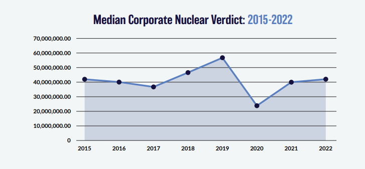

Let’s start by looking at exactly what the chart is showing - in this context, a ‘nuclear verdict’ is defined as a US corporate civil verdict, which exceeds a fixed dollar value of $10m. You should hopefully be aware (for example see the paper by Brazauskas et al. (2009)) [1] that as a measure of trend, examining the increase in average claim excess of a fixed dollar threshold does not accurately reflect the underlying trend. It can be geared so as to cause a ‘greater than underlying’ trend, and it can also be less than the underlying trend (or even give a value of 0) depending on the exact shape of the distribution. For example, if our underlying trend is 8%, then the increase in average claim excess $10m may present itself in the data as 12%, as 4%, or even as 0% depending on the exact shape of the data. And this is not a ‘lack of data’ issue, i.e. the real answer will converge over time with more data, there is an inherent bias in the methodology.

The intuition behind the phenomenon is that we might have a whole bunch of losses just under the threshold, which when inflated are pushed to just above the threshold, and thereby adding a whole load of new small claims, bringing down the average of the losses above the threshold.

To be exact, the paper by Brazauskas et al. referenced above, shows that analysing the *mean* excess value does not accurately reflect trend, but our chart uses the *median* excess value. The obvious follow up question is does the median also have the same issue as the mean? Intuitively, the same arguments relating to verdicts just under the threshold seems to apply, but let’s run a quick python script to check.

The following script runs 50k monte carlo simulations, each simulation generates values from a lognormal distribution. We then inflate the simulated values by 5% pa, and then restrict ourselves to just the 'nuclear' verdicts, i.e. those above the threshold of 10m. Finally we analyse the median of these nuclear verdicts and assess the trend in the median over time. Here's our Python code:

In [1]:

import numpy as np
import pandas as pd
import scipy.stats as scipy
from math import exp
from math import log
from math import sqrt
from scipy.stats import lognorm
from scipy.stats import poisson
from scipy.stats import linregress

In [2]:

Distmean = 10000000.0
DistStdDev = Distmean*1.5
AverageFreq = 100
years = 10
ExposureGrowth = 0.0

Mu = log(Distmean/(sqrt(1+DistStdDev**2/Distmean**2)))
Sigma = sqrt(log(1+DistStdDev**2/Distmean**2))

LLThreshold = 1e7
Inflation = 0.05

s = Sigma
scale= exp(Mu)

In [3]:

MedianLL = []
AllLnOutput = []

for sim in range(50000):

    SimOutputFGU = []
    SimOutputLL = []
    year = 0
    Frequency= []
    for year in range(years):
        FrequencyInc = poisson.rvs(AverageFreq*(1+ExposureGrowth)**year,size = 1)
        Frequency.append(FrequencyInc)
        r = lognorm.rvs(s,scale = scale, size = FrequencyInc[0])
        r = np.multiply(r,(1+Inflation)**year)
        r = np.sort(r)[::-1]
        r_LLOnly = r[(r>= LLThreshold)]
        SimOutputFGU.append(np.transpose(r))
        SimOutputLL.append(np.transpose(r_LLOnly))
        
    SimOutputFGU = pd.DataFrame(SimOutputFGU).transpose()
    SimOutputLL = pd.DataFrame(SimOutputLL).transpose()    
    a = np.log(SimOutputLL.median())
    AllLnOutput.append(a)
    b = linregress(a.index,a).slope
    MedianLL.append(b)

AllLnOutputdf = pd.DataFrame(AllLnOutput)

dfMedianLL = pd.DataFrame(MedianLL)
dfMedianLL['Exp-1'] = np.exp(dfMedianLL[0]) -1
print(np.mean(dfMedianLL['Exp-1']))
print(np.std(dfMedianLL['Exp-1']))

0.01414199139951309
0.013860637023388517

In [ ]:

The value of 1.4% we have outputted at the bottom is the average trend in the median of the nuclear verdicts. We can see that based on this analysis, even though we know that the underlying data has a trend of 5%, the median of the values greater than 10m, only increases by 1.4% pa.

What could we have done instead? We could have analysed the median of the top X verdicts, where X could for example be 10, 20, 50, 100. For a write up of this method, see the following:
www.lewiswalsh.net/blog/backtesting-inflation-modelling-median-of-top-x-losses