Modelling Extremal Events - Cramer-Lundberg theorem under LogN

3/11/2023

I’ve had the textbook 'Modelling Extremal Events: For Insurance and Finance’ sat on my shelf for a while, and last week I finally got around to working through a couple of chapters. One thing I found interesting, just around how my own approach has developed over the years, is that even though it’s quite a maths heavy book my instinct was to immediately build some toy models and play around with the results. I recall earlier in my career, when I had just got out of a 4-year maths course, I was much more inclined to understand new topics via working through proofs step-by-step in long hand, pen to paper.

In case it’s of interest to others, I thought I’d upload my Excel version I built of the classic ruin process. In particular I was interested in how the Cramer-Lundberg theorem fails for sub-exponential distributions (which includes the very common Lognormal distribution). Therefore the Spreadsheet contains a comparison of this theorem against the correct answer, derived from monte carlo simulation.

The Speadsheet can be found here:
https://github.com/Lewis-Walsh/RuinTheoryModel

The first tab uses an exponential distribution, and the second uses a Lognormal distribution. Screenshot below.

I also coded a similar model in Python via Jupyter Notebook, which you can read about below.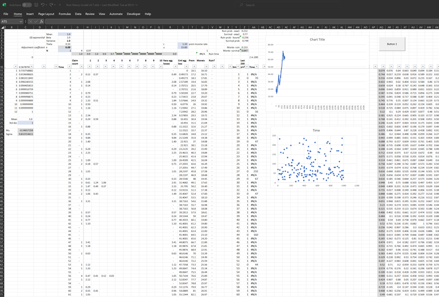

Here I have specifically used a LogN distribution, and I compare the ruin probability I derive using a monte carlo simulation, with the value from the Cramer-Lundberg theorem, to understand the extent to which it under-estimates the ruin probability.

In [1]:

import numpy as np
import time
import matplotlib.pyplot as plt
import math

In [2]:

# Set parameters
mean_poisson = 1
mean_lognormal = 1
std_dev_lognormal = 1.5
u = 15
c = 1.1
num_simulations = 10000
max_poisson_samples = 500

# Calculate parameters mu and sigma
mu = np.log(mean_lognormal**2 / np.sqrt(std_dev_lognormal**2 + mean_lognormal**2))
sigma = np.sqrt(np.log(1 + std_dev_lognormal**2 / mean_lognormal**2))

In [3]:

# Initialize arrays to record results
results = []
poisson_sims_before_stop = []

# Start timing for simulations
start_time_simulations = time.time()

for _ in range(num_simulations):
    t = 0
    S_t = 0
    poisson_sims = 0
    
    while t < max_poisson_samples:
        poisson_sample = np.random.poisson(mean_poisson)
        lognormal_samples = np.random.lognormal(mu, sigma, poisson_sample)
        S_t += np.sum(lognormal_samples)
        
        f_t = u + c*t - S_t
        
        if f_t < 0:
            results.append(1)
            poisson_sims_before_stop.append(poisson_sims)
            break
        
        t += 1
        poisson_sims += 1
    
    if t == max_poisson_samples:
        results.append(0)
        poisson_sims_before_stop.append(poisson_sims)

In [4]:

# Filter out values less than max_poisson_samples (500)
filtered_poisson_sims = [sims for sims in poisson_sims_before_stop if sims < max_poisson_samples]

# Calculate average number of Poisson simulations before stopping
avg_poisson_sims = np.mean(filtered_poisson_sims)

#Calculate the ruin probability
ruin_prob = len(filtered_poisson_sims) / len(poisson_sims_before_stop)

# Calculate total execution time in minutes and seconds
end_time_total = time.time()
execution_time_total = end_time_total - start_time_simulations
minutes_total = int(execution_time_total // 60)
seconds_total = int(execution_time_total % 60)

In [5]:

print(f"Ruin probability - monte carlo")
print(ruin_prob)

print(f"Ruin probability - Cramer-Lundberg")
theta = c/(mean_poisson*mean_lognormal)-1
print(1/(1+theta)*math.exp((-1*theta*u)/(1+theta)))

# Create a histogram to visualize the distribution
plt.hist(filtered_poisson_sims, bins=30, density=True, alpha=0.6, color='g', edgecolor='black')
plt.xlabel('Number of Poisson simulations before stopping')
plt.ylabel('Frequency')
plt.title('Distribution of Poisson Simulations Before Stopping')
plt.show()

Ruin probability - monte carlo
0.3703
Ruin probability - Cramer-Lundberg
0.23248105446645487

In [ ]:

We see the output from the Monte Carlo and Cramer-Lundberg (CL) at the bottom. The monte carlo is our 'correct' value and gives us a 37% chance of ruin, whereas the CL method only thinks there is a 23% chance of ruin. So, by using the CL method, we'd be quite materially underestimating the risk of ruin.

Modelling Extremal Events - Cramer-Lundberg theorem under LogN

Leave a Reply.

Author

Sign up to get updates when new posts are added

Categories

Archives