
In which we plot an excessive number of graphs, fix our problems with null values, re-run our algorithm, and significantly improve our accuracy. Source: https://somewan.design We made a fairly strong start last time, we started a new problem - predicting house prices - did some data exploration, and got a first cut of a model set up. The main task for today is to do some more data exploration, which will hopefully lead on to some new ideas about how to improve our model. One approach that I'm already considering, is to just chuck in as many variables as possible and see what happens. Mobile users - once again, if the section below is not rendering well, then please consider rotating to landscape view to see if that improves the layout. I've also made a few changes to the layout of the final which will hopefully help somewhat.
In [1]:
import os
import numpy as np
import matplotlib.pyplot as plt
import pandas as pd
from sklearn.ensemble import RandomForestRegressor
In [2]:
path = "C:\Work\Machine Learning experiments\Kaggle\House Price"
os.chdir(path)
In [3]:
train_data = pd.read_csv("train.csv")
test_data = pd.read_csv("test.csv")
In [4]:
# I'm using this instead of the head command as it renders better for mobile users

train_data.iloc[1:,1:5]
Out[4]:
1459 rows × 4 columns
In [5]:
TrainColumns = train_data.columns
train_data.columns
Out[5]:
Index(['Id', 'MSSubClass', 'MSZoning', 'LotFrontage', 'LotArea', 'Street',
       'Alley', 'LotShape', 'LandContour', 'Utilities', 'LotConfig',
       'LandSlope', 'Neighborhood', 'Condition1', 'Condition2', 'BldgType',
       'HouseStyle', 'OverallQual', 'OverallCond', 'YearBuilt', 'YearRemodAdd',
       'RoofStyle', 'RoofMatl', 'Exterior1st', 'Exterior2nd', 'MasVnrType',
       'MasVnrArea', 'ExterQual', 'ExterCond', 'Foundation', 'BsmtQual',
       'BsmtCond', 'BsmtExposure', 'BsmtFinType1', 'BsmtFinSF1',
       'BsmtFinType2', 'BsmtFinSF2', 'BsmtUnfSF', 'TotalBsmtSF', 'Heating',
       'HeatingQC', 'CentralAir', 'Electrical', '1stFlrSF', '2ndFlrSF',
       'LowQualFinSF', 'GrLivArea', 'BsmtFullBath', 'BsmtHalfBath', 'FullBath',
       'HalfBath', 'BedroomAbvGr', 'KitchenAbvGr', 'KitchenQual',
       'TotRmsAbvGrd', 'Functional', 'Fireplaces', 'FireplaceQu', 'GarageType',
       'GarageYrBlt', 'GarageFinish', 'GarageCars', 'GarageArea', 'GarageQual',
       'GarageCond', 'PavedDrive', 'WoodDeckSF', 'OpenPorchSF',
       'EnclosedPorch', '3SsnPorch', 'ScreenPorch', 'PoolArea', 'PoolQC',
       'Fence', 'MiscFeature', 'MiscVal', 'MoSold', 'YrSold', 'SaleType',
       'SaleCondition', 'SalePrice'],
      dtype='object')
In [6]:
# Let's just go ahead and graph all 80 variables against sale price:
# I think this will be instructive in terms of being intuition

fig = plt.figure()
fig.subplots_adjust(hspace=0.5, wspace=0.5)
fig.set_figheight(18)
fig.set_figwidth(18)
for i in range(1,10):
    TempPivot = train_data.groupby(TrainColumns[i])['SalePrice'].mean().sort_values()
    ax = fig.add_subplot(3,3,i)
    ax = TempPivot.plot.bar()

In [7]:
fig = plt.figure()
fig.subplots_adjust(hspace=0.5, wspace=0.5)
fig.set_figheight(18)
fig.set_figwidth(18)
for i in range(11,20):
    TempPivot = train_data.groupby(TrainColumns[i])['SalePrice'].mean().sort_values()
    ax = fig.add_subplot(3,3,i-10)
    ax = TempPivot.plot.bar()

In [14]:
# Okay that was all of them. The categorical ones rendered well, the numerical ones less so
# but we can still see the overall shape of the relationship.

# What is our takeaway from this? - generally most of the variables look pretty useful!

# As a next step, let's try to just chuck all variables into the Random Forest algorithm and
# see what happens. Since most of them seem to differentiate the sale price, I'm hoping
# this will lead to an increase in accuracy.

# According to things I've read online, the Random Forest algorithm is fairly (but not completely)
# robust to Outliers, Multicollinarity, and non-linearity. So I'm not going to adjust for these
# issues now, but we can possibly return to this at a later stage and see if it helps.

# [Message from the future] - tried to use all variables in the Random Forest, but this threw up
# an error due to the presense of null values in some of the columns. We therefore need to add
# a step where we remove all columns which have a null value, and just fit against what is left
In [15]:
train_data.columns
features = []
In [16]:
frames = [train_data, test_data]

Total_data =  pd.concat(frames)
Total_data.iloc[1:,1:5]
Out[16]:
2918 rows × 4 columns
In [17]:
# We are now running through all columns, if a null value is found, add it to
# the featuresNotUsed list, otherwise put it in the features list

TrainColumns
features = []
featuresNotUsed = []

for i in TrainColumns:
    if not(Total_data[i].isnull().values.any()):
        if not(i == 'Id'):
            if not(i == 'SalePrice'):
                features.append(i)
    else:
        featuresNotUsed.append(i)

features
Out[17]:
['MSSubClass',
 'LotArea',
 'Street',
 'LotShape',
 'LandContour',
 'LotConfig',
 'LandSlope',
 'Neighborhood',
 'Condition1',
 'Condition2',
 'BldgType',
 'HouseStyle',
 'OverallQual',
 'OverallCond',
 'YearBuilt',
 'YearRemodAdd',
 'RoofStyle',
 'RoofMatl',
 'ExterQual',
 'ExterCond',
 'Foundation',
 'Heating',
 'HeatingQC',
 'CentralAir',
 '1stFlrSF',
 '2ndFlrSF',
 'LowQualFinSF',
 'GrLivArea',
 'FullBath',
 'HalfBath',
 'BedroomAbvGr',
 'KitchenAbvGr',
 'TotRmsAbvGrd',
 'Fireplaces',
 'PavedDrive',
 'WoodDeckSF',
 'OpenPorchSF',
 'EnclosedPorch',
 '3SsnPorch',
 'ScreenPorch',
 'PoolArea',
 'MiscVal',
 'MoSold',
 'YrSold',
 'SaleCondition']
In [18]:
featuresNotUsed
Out[18]:
['MSZoning',
 'LotFrontage',
 'Alley',
 'Utilities',
 'Exterior1st',
 'Exterior2nd',
 'MasVnrType',
 'MasVnrArea',
 'BsmtQual',
 'BsmtCond',
 'BsmtExposure',
 'BsmtFinType1',
 'BsmtFinSF1',
 'BsmtFinType2',
 'BsmtFinSF2',
 'BsmtUnfSF',
 'TotalBsmtSF',
 'Electrical',
 'BsmtFullBath',
 'BsmtHalfBath',
 'KitchenQual',
 'Functional',
 'FireplaceQu',
 'GarageType',
 'GarageYrBlt',
 'GarageFinish',
 'GarageCars',
 'GarageArea',
 'GarageQual',
 'GarageCond',
 'PoolQC',
 'Fence',
 'MiscFeature',
 'SaleType',
 'SalePrice']
In [19]:
Y = train_data['SalePrice']
In [20]:
X = pd.get_dummies(train_data[features])
X_test = pd.get_dummies(test_data[features])
In [21]:
#The below is just copy and pasted from the Titanic challenge. We're making
# Sure that all our variables are in both the test and train set, otherwise
# we'll get errors. It's nice to have built up a few code snippets I can just
# copy and paste without having to reininvent the wheel

columns = X.columns
ColList = columns.tolist()


missing_cols = set( X_test.columns ) - set( X.columns )
missing_cols2 = set( X.columns ) - set( X_test.columns )
# Add a missing column in test set with default value equal to 0
for c in missing_cols:
    X[c] = 0

for c in missing_cols2:
    X_test[c] = 0
# Ensure the order of column in the test set is in the same order than in train set
X = X[X_test.columns]
In [22]:
X.iloc[1:,1:5]
Out[22]:
1459 rows × 4 columns
In [23]:
X_test.iloc[1:,1:5]
Out[23]:
1458 rows × 4 columns
In [24]:
RFmodel = RandomForestRegressor(random_state=1)
RFmodel.fit(X,Y)
predictions = RFmodel.predict(X_test)
In [56]:
output = pd.DataFrame({'ID': test_data.Id, 'SalePrice': predictions})
output.to_csv('my_submission - V2 - RF.csv',index=False)
So all that remains is to upload our submission and see how we performed. 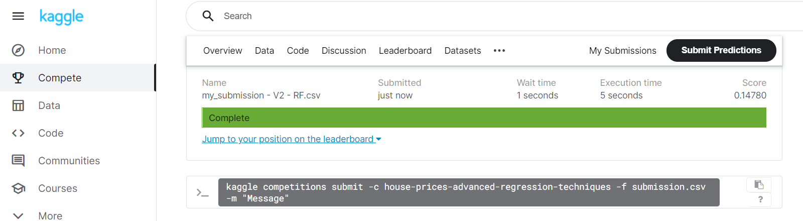
And voila! We've improved our score from approx 0.2 down to 0.14780, moving us up to 2830 out of 4891 entries. Tune in next time when we do some more data cleansing, deal with those pesky null values, and marginally improve our model. |
AuthorI work as an actuary and underwriter at a global reinsurer in London. Categories
All
Archives
April 2024
|
 RSS Feed
Leave a Reply.