An Actuary learns Machine Learning – Part 5 – lots of machine learning models

In which we take our final stab at the titanic challenge by ‘throwing the kitchen sink’ at the problem, setting up another 5 different machine learning models and seeing if they improve our performance (hint they do not, but hopefully it's still interesting)
​


​
​Source: https://somewan.design

---

Today we've got a fairly straightforward task, all we are going to do is get a few more machine learning algorithms set up on our titanic dataset, and see how they perform relative to our current models. We did most of the hard work getting the data into a useable format - encoding categorical variables, dealing with blank or incomplete values, etc - this should be the easy fun bit now.

The models we will use are:

• Logistic Regression
• Support Vector Machine
• K-Nearest Neighbour
• Gaussian Naïve Bayesian
• Perceptron

We could use a neural network as well, but they look much more complicated to set up, so I decided to skip it for now.

At this stage you might be asking yourself 'why are there so many models we can use, and which is the best model'? All the models do basically the same thing - they are supervised learning algorithms, in this case used for a classification problem. Each algorithm approaches the problem in a slightly different way, and each has it's strengths and weaknesses. So it doesn't really make sense to ask which is the 'best'. They're all different, and the 'best' one is the one which is the most useful, all things considered. In other words, there's no getting around us having to try them all out on the problem.

So, first up - let's try Logistic Regression, a type of GLM which uses the logistic function as a link function:

Input:

LGmodel = LogisticRegression()
LGmodel.fit(X,Y)
predictions = LGmodel.predict(X_test)

​Output: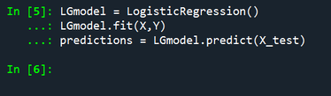

And that’s it! In just three lines of code, we've referenced a new model, fit it against our data, and then used it to predict against the test set. One thing that’s been eye-opening about learning some of these tools and algorithms, is how easy other people have made it to run these models. Everything seems to just works out of the box first time, it’s great.

Like a trashy reality tv show, I’m going to build some suspense and not show the results table until the end. So we won't see how Logisitc Regression performed until the big reveal at the end.

Next up, let's get a Support Vector Machine working:
​
Input:

svc = SVC()
svc.fit(X, Y)
predictions = svc.predict(X_test)

​Output: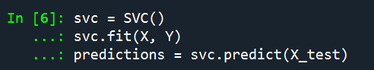

You may be able to spot immediately, the code is:

• Short
• Easy to follow
• The exact syntax of the Logistic Regression function

They really have made it easy for us.
​
Input:

knn = KNeighborsClassifier(n_neighbors = 3)
knn.fit(X, Y)
predictions = knn.predict(X_test)

Output: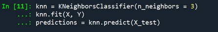
​

Input:

Gaussian = GaussianNB()
gaussian.fit(X, Y)
predictions = gaussian.predict(X_test)

​Output: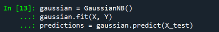

Input:

perceptron = Perceptron()
perceptron.fit(X, Y)
predictions = perceptron.predict(X_test)

​Output: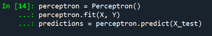

​And that is it, we’ve ran all our models, all we need to do now is output the predictions, and see how they have performed. And here is our final table: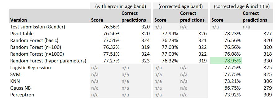

So even though we’ve set up all these additional models, none of them appear to have worked very well! Let’s just look at the final columns, and sort best to worst:

​

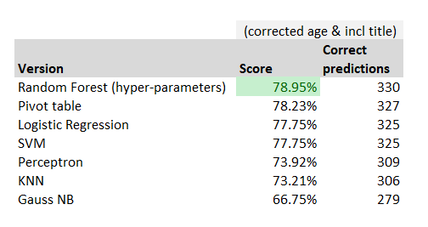
So the winner was the Random Forest algorithm with hyper-parameter tuning, in second place was actually our trusty pivot table model, Logisitc Regression and SVM were joint third, and we quickly drop off then with the final three models we ran.

It’s possible the other models could have been improved if we’d also ran some version of hyper-parameter tuning on them, just using out-the-box Random Forests gave a similar performance to the out-the-box Logistic Regression and Support Vector Machine.

Summary

So that’s it for the Titanic challenge, there is a lot more we could have done, however I’m keen to move on and play around with a new data set. So what can we take away from what we’ve done in the last 5 posts?

I’m definitely going to use some of these tools when tackling actuarial problems, I think the ideas around cross validation, and using a training/test set are great. We often talk about not over-fitting actuarial models, however the way I’ve seen that play out in practice is either as a fairly lazy excuse for always using a lognormal distribution (but it’s heavy tailed when sigma is large!, etc.), or possibly only fitting against some of the more common distributions when parameterising a severity curve in curve fitting software. (For an exception to this, and in hindsight an approach that does take on board these lessons, see Chhabra and Parodi 2010).
​
Another take away for me is that the models themselves are super easy to set up and use, and can clearly outperform simple heuristic based approaches. Next time I’ve got a big enough dataset I’m definitely going to try some of these out. Some of these models (logistic regression for example) can be seen as special cases of GLMs, so maybe I’m just showing my bias in that I’m not sufficiently familiar with GLMs, having come from a London Market reinsurance background rather than a Personal Lines background.

A final thought, is that all the well written tutorials I read online used inventive and thoughtful data visualisation – they projected higher-dimension datasets onto 2-d planes, they used visualisations to understand the difference between the predictions of two models, and they even managed to convey family groupings. Here are some of the better visualisations:

Family groupings in on chart with survival/death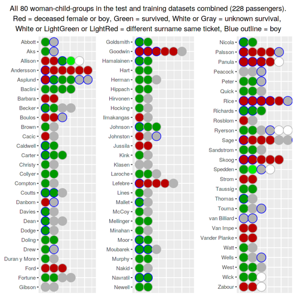

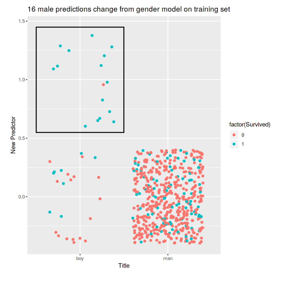
Understanding the difference in predications made between two models:

2-d projection of higher-dimension data

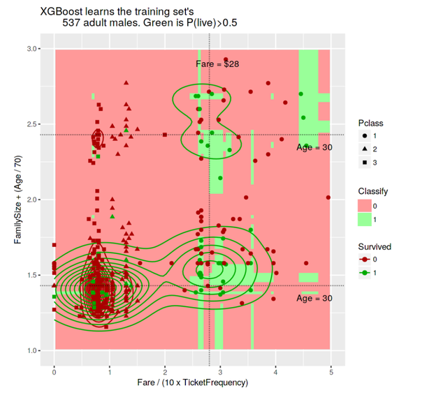
​There is clearly a ton of structure and information in this graph, and it can be so useful getting everything into one image to allow us to understand this structure.
 
So that’s all folks, tune in next time when we move on to our next challenge – the Kaggle House Price prediction challenge, where we will attempt to apply everything we learned to solve this new problem, and hopefully pick up some new tricks on the way!